5kN Methalox Rocket Engine

Introduction

I love rocket engine, this is one of my main study and focus. Rocket engine is one of the peak of human technology. That’s why, to implement what I know and to learn more about rocket engine, not only the textbook theory, but also the the systems, components, how the design choice influence the performance, etc; I create this project.

First of all, I learned about rocket engine and have interest on it since 2022. I read a book: Rocket Propulsion Element to know the history, aerodynamics and thermodynamics behind it, how to evaluate the rocket performance, some kind of rocket engine configurations, and so on. That’s how I built my serious interest on a rocket engine. That’s why, in this project, I think I wanna discuss about why I choose “this specific component” instead of others, how the analysis and equation I used, and how I analysed each component step by step.

First of all, why 5kN? Yeah, basically 5kN rocket engine categorized as a small, home-made rocket engine. Every rocket enthusiast or rocket engineer could build their own 5kN rocket engine in their garage. And, I start from the simple one. Yeah, that’s how I thought at the first time. Complicated things happened after it. So, I start from 5 kN rocket engine because I thought it was simple.

Why Methalox? Well, first because I thought it cool and spaceX use it for their rocket. I considered RP-1 (kerosene + Lox) too, but then, after I do some study case, and learn about some propellant characteristics, I choose methalox for some different reasons. First, Methalox offers higher specific impulse. Specific impulse can be calculated as:

I_{sp}=\frac{v_e}{g_0}=\frac{1}{g_0}\sqrt{\frac{2k}{k-1}\frac{RT_c}{M}\left[1-\left(\frac{P_e}{P_c}\right)^{\frac{k-1}{k}}\right]}

Tc is combustion chamber temperature, M is average molecular weight of the exhaust gas, and Pc and Pe are chamber and exit pressure respectively. Then, you can see to the molecular weight denominator here, for higher Isp, you need lower molecular weight. And methalox exhaust mostly water vapor ( $H_2O$ ) offers lower molecular weight (18 g/mol) compared to kerosene exhaust that heavily contains carbon dioxide (CO2) (44g/mol). 2nd reason is because kerosene produce soot that possibly causes coking and potentially destroy the engine efficiency. Theoritically, methalox offers Isp = 380 second in vacuum compared to 330 second for kerolox.

Why kerolox producing soot so much? Well, we can see the chemical equilibrium:

CH_4+2O_2\rightarrow CO_2+2H_2O

C_{12}H_{24}+18O_2\rightarrow 12CO_2+12H_2O

Then we can consider the carbon-to-hydrogen (C:H) ratio for each fuel. Rocket engine purposely run fuel rich to lower the chamber temperature and protect the wall of the inner thrust chamber wall.

C\!:\!H_{ratio}=\frac{\text{mass of carbon}}{\text{mass of hydrogen}}

For methane, the ratio is 3, and for kerosene the ratio is 6. Kerosene has double the carbon mass per hydrogen atom compared to methane. When running fuel-rich, those excess unbonded carbon atoms in kerosene instantly form solid soot deposits (coking). Methane’s low carbon-to-hydrogen ratio ensures that even during fuel-rich cycles, the carbon stays bound in gaseous forms, keeping the engine clean for rapid reuse.

After I decided the thrust and the fuel, I move on to the operating conditions. Here I did trade off study. First, I look at raptor engine with 300 bar pressure. Ended up with a very small rocket engine (because for the same thrust, higher your chamber pressure resulting smaller engine size). This trade off can be studied by the following equations:

F=C_fP_cA_t

C_f=\sqrt{\frac{2k^2}{k-1}\left(\frac{2}{k+1}\right)^{\frac{k+1}{k-1}}\left[1-\left(\frac{P_e}{P_c}\right)^{\frac{k-1}{k}}\right]}

The correlation clearly can be seen on the figure below.

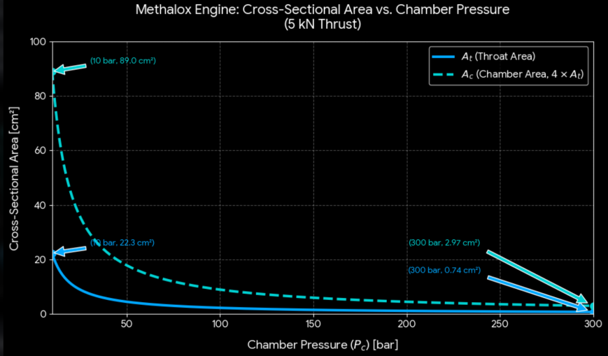
Graph showing the correlation between combustion-chamber pressure and throat or combustion-chamber area.

Figure 1. Chamber pressure to area correlation.

38 bar is the sweet spot between the size, material characteristics, and, the possibility to build.

Nozzle shape is the next crucial component to decide. There are several nozzle designs exist today such as bell nozzle, conical shape, aerospike, or expansion deflection (as you can see on the figure 2) with bell nozzle is the most common used configuration. Two things need to ensure and consider here are that we make the nozzle not merely to get the maximum performance (by ensuring there’s no underexpanded/overexpanded area), but also need to consider the manufacturing process. Half contoured/bell shape nozzle offers the highest theoretical efficiency, but its hard to manufactured can only manufactured using additive material technique such as metal 3D printing. In Indonesia especially, this kind of technology is new and I have no access to it. So, I decide to use conical shape based on that consideration. It’s easier to manufactured and the performance loss is only 2% theoretically. So, it’s the sweet spot.

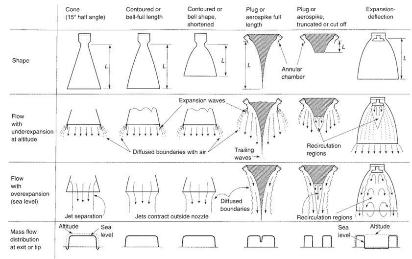
Comparison of conical, bell, annular, expansion-deflection, and plug nozzle shapes.

Figure 2. Nozzle shapes [1]

After deciding the nozzle shape, it’s time to move on to the material selection. There are several common materials used today for rocket engine, Inconel, copper alloys, tungsten, etc. Inconel is hard to access, as long as tungsten. After I look at the characteristics for some materials, I decide to choose copper alloy. But, there are a lot of copper alloy materials such as C12200, c10200, and CuCrCz. Ofc CuCrCz is the most commonly used copper alloy material in rocket engine, but it’s for high pressure-high performance rocket engine with more than 50 bar chamber pressure. Mine, on the other hand, is only 38 bar. C10200 offers an excellent thermal conductivity, higher than CuCrCz with a lower strength compromise. To decide which one I need to go with, I did some calculations using NASA CEA to know especially the hot gas combustion chamber temperature. I got a value around 3300K. Then, from the analytical calculation using numerical model with some equations from modern engineering for design of liquid propellant rocket engines book [2].

Heat Transfer Calculation

I realized that it’s impossible for me to completely ignoring film cooling technique. My thrust chamber would absolutely melting down just in few seconds. So, from the first time, I decide to combine regenerative cooling and film cooling technique. Several equations I used as follow.

q_w=\alpha_T(T_e-T_w)

Where,

T_e=T_c^0\left[\frac{1+Pr^{0.33}\left(\frac{\gamma-1}{2}\right)M^2}{1+\left(\frac{\gamma-1}{2}\right)M^2}\right]

For the heat transfer coefficient, the following correlation is used.

\alpha_T=\left[\frac{0.026(\mu_\infty^0)^{0.2}C_{p\infty}^0}{D_t^{0.2}(Pr_\infty^0)^{0.6}}\left(\frac{P_c^0}{c^*}\right)^{0.8}\left(\frac{D_t}{R}\right)^{0.1}\left(\frac{A_t}{A}\right)^{0.9}\right]\sigma

The correction factor $\sigma$ can be calculated as follows:

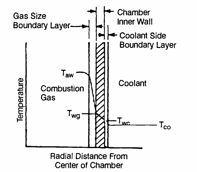
\sigma=\left[\frac{1}{2}\frac{T_w}{T_c^0}\left(1+\frac{\gamma-1}{2}M^2\right)+\frac{1}{2}\right]^{-0.68}\left[1+\frac{\gamma-1}{2}M^2\right]^{-0.12}

Temperature profile across the gas-side boundary layer, chamber wall, coolant-side boundary layer, and coolant.

Figure 3. regenerative cooling and film cooling technique

We need one more equation for the film cooling, the boundary layer cooling. I use some assumptions below to calculate the boundary layer cooling:

The large-scale distribution of mixture composition and the gas properties in the shear flow are conserved along the nozzle.
The convective heat flux to the wall is completely defined by the heat transfer between the wall and the layer next to the wall.
The layer next to the wall is transparent for the radiation heat transfer.

To calculate the convective heat flux from the cooler surface layer, the Levlev’s correlation for similar conditions is used

\frac{q^{(1)}}{q^{(2)}}=\frac{S^{(1)}}{S^{(2)}}

Where,

S=\frac{(I_\infty^0-I_w)T_e^{0.425}\mu_{1000}^{0.15}}{R_{1500}^{0.425}(T_e+T_w)^{0.595}(3T_e+T_w)^{0.15}}

I also consider the radiation effect, which is, for given hot gas temperature $T_\infty$ and wall temperature $T_w$ , the basic correlation for the radiation heat transfer is given by,

q_r=\varepsilon_e\sigma\left(\varepsilon_r^{T_\infty}T_\infty^4-\varepsilon_g^{T_w}T_w^4\right)

Where $\sigma$ is Stefan boltzman constant and $\varepsilon$ is the emissivity.

Radiation is not only a heat load coming from the combustion gas, it is also the way the wall throws energy back out through its outer surface. Putting the two together gives the thermal balance the wall has to satisfy in steady state, and for the cooled thrust chamber I wrote it as:

q_w^{T_{wg}}+q_r^{T_{wg}}=\frac{\lambda_w}{t_w}(T_{wg}-T_{wc})=\varepsilon_{wc}\sigma T_{wc}^4=q_{rc}^{T_{wc}}

where

$q_w^{T_{wg}}$ and $q_r^{T_{wg}}$ are the convective and the radiation heat flux arriving at the inner surface of the wall, both taken at the inner wall temperature $T_{wg}$ ;

$q_{rc}^{T_{wc}}$ is the radiation heat flux leaving the outer surface of the wall at the outer wall temperature $T_{wc}$ ;

$T_{wg}$ is the temperature of the inner (gas-side) wall surface;

$T_{wc}$ is the temperature of the outer wall surface;

$\sigma=5.670373\times10^{-8}\ \mathrm{W/(m^2K^4)}$ is the Stefan–Boltzmann constant;

$\varepsilon_{wc}$ is the emissivity coefficient of the wall material, taken at the outer surface temperature;

$\lambda_w$ is the thermal conductivity of the wall, evaluated at the mean wall temperature $T=0.5(T_{wg}+T_{wc})$ ;

$t_w$ is the thickness of the wall.

Because both wall temperatures sit on every side of this balance, it cannot be solved in one shot. I solve it iteratively at each chamber and nozzle station, and the loop stops as soon as a pair of $T_{wg}$ and $T_{wc}$ is found for which the heat flux entering the inner surface, $(q_w^{T_{wg}}+q_r^{T_{wg}})$ , equals the flux radiated away from the outer surface, $q_{rc}^{T_{wc}}$ .

After that, I also consider regenerative cooling. I use the following equations,

q_w^{T_{wg}}+q_r^{T_{wg}}=\dot{m}_c\bar{c}_c(T_c^{out}-T_c^{in})

q_w^{T_{wg}}+q_r^{T_{wg}}=\alpha_c(T_{wc}-T_c)

\alpha_c=\frac{Nu\lambda_c}{d_e}

For methane,

Nu=0.0185Re_c^{0.8}Pr_c^{0.4}\left(\frac{T_c}{T_{wc}}\right)^{0.1}

The result can be seen in the figure 1. This is the wall-gas temperature and the regenerative cooling temperature along the burner.

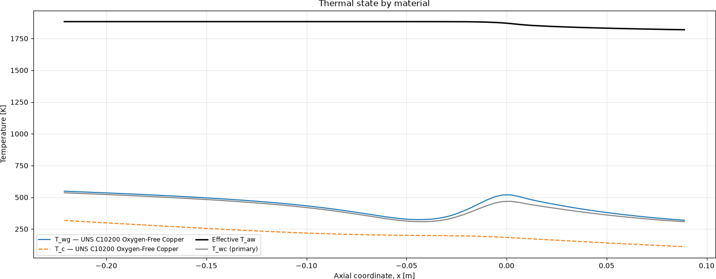
Gas-side wall temperature and regenerative coolant temperature plotted along the axial coordinate.

Figure 4. gas-side wall temperature and regenerative coolant temperature.

Analytical Calculation and Inhouse Program

We can’t simply create this 3D view. Preliminary analytical calculation can be used to know the thrust chamber geometry, regenerative cooling sizing, and the wall thickness. But, when it turns into a 3D design, we have to ensure that everything are well calculated. For example, the area of the manifold. Manifold have to design to has space larger than the regenerative cooling channel. Then, the inlet manifold. We have to design it with appropriate massflow and velocity magnitude so we don’t accidentally make it chocked. Every hole, every component must be created with their specific calculation and objective. I can’t show the detailed calculation here because it would make this content to be soo long.

The objective of this 3D model is for the simulation requirement. Ofc I’ve done the analytical calculation, and built my own program for it, and analysed it using CEA. However, high fidelity CFD simulation was still needed (who do not want to see those cool diamond shock contour? Haha). So, yeah I did it. Because I can’t simulate it spontaneously and iterate the thickness of the rocket thrust chamber (so expensive). So I conducted an analytical calculation and create a program to calculate the thermal and pressure stress. I modelled the burner as a global axisymmetric model with a thickness $t_{eff}$ . $t_{eff}$ is either a hot wall ligament thickness or the smooth-wall thickness.

r(x,\eta)=r_i(x)+\eta t_{eff}(x)

Each mapped quadrilateral is split into two three-node linear triangles.

Then I applied temperature to the structural mesh. First I did a linear mapping:

f_{lin}(x,r)=\frac{r-r_i(x)}{r_o(x)-r_i(x)}

T(x,r)=T_{wg}(x)+f_{lin}(x,r)[T_{wc}(x)-T_{wg}(x)]

For the cylinder shape:

f_{cyl}(x,r)=\frac{\ln\left(\frac{r}{r_i(x)}\right)}{\ln\left(\frac{r_o(x)}{r_i(x)}\right)}

T(x,r)=T_{wg}(x)+f_{cyl}(x,r)[T_{wc}(x)-T_{wg}(x)]

Then the axisymmetric displacement and strain can be calculated as, every node has 2 degrees of freedom

u_i= \begin{bmatrix} u_x\\ u_r \end{bmatrix}_i

The strain vector is ordered as,

\varepsilon= \begin{bmatrix} \varepsilon_r\\ \varepsilon_\theta\\ \varepsilon_x\\ \gamma_{rx} \end{bmatrix}

With

\varepsilon_r=\frac{\partial u_r}{\partial r}; \qquad \varepsilon_\theta=\frac{u_r}{r}; \qquad \varepsilon_x=\frac{\partial u_x}{\partial x}; \qquad \gamma_{rx}=\frac{\partial u_x}{\partial r}+\frac{\partial u_r}{\partial x}

For three-node triangle with shape function $N_i$ ,

u_x=\sum_{i=1}^{3}N_i u_{x,i}; \qquad u_r=\sum_{i=1}^{3}N_i u_{r,i}

$\varepsilon$ can be calculated as,

\varepsilon= \begin{bmatrix} 0&N_{1,r}&0&N_{2,r}&0&N_{3,r}\\ 0&N_1/r&0&N_2/r&0&N_3/r\\ N_{1,x}&0&N_{2,x}&0&N_{3,x}&0\\ N_{1,r}&N_{1,x}&N_{2,r}&N_{2,x}&N_{3,r}&N_{3,x} \end{bmatrix} \begin{bmatrix} u_{x,1}&u_{r,1}&u_{x,2}&u_{r,2}&u_{x,3}&u_{r,3} \end{bmatrix}^{T}

Then, from those shape functions, we need their derivatives. For the triangle coordinates (xᵢ, rᵢ), the signed double area is:

2A=(x_2-x_1)(r_3-r_1)-(x_3-x_1)(r_2-r_1)

Yeah, because the triangle is linear, the derivatives are constant inside each element. So I don’t need to re-evaluate them for every integration point, I just calculate them once per triangle:

\frac{\partial N}{\partial x} = \frac{1}{2A} \begin{bmatrix} r_2-r_3\\ r_3-r_1\\ r_1-r_2 \end{bmatrix}

\frac{\partial N}{\partial r} = \frac{1}{2A} \begin{bmatrix} x_3-x_2\\ x_1-x_3\\ x_2-x_1 \end{bmatrix}

Degenerate or negatively oriented triangles (2A ≤ 0) are rejected. This one is important, because a flipped or zero-area triangle gives a negative volume weight and silently poisons the whole stiffness matrix. Better to kill it early than to trust a good looking result that is actually wrong.

Next, the material matrix. One thing I don’t want to do is treating the copper as a constant-property material, because my wall lives between cryogenic methane on the coolant side and hundreds of Kelvin on the gas side. Copper loses stiffness and expands differently along that range. So, at every integration point, the program evaluates:

E=E(T),\qquad \nu=\nu(T),\qquad \alpha=\alpha(T)

Then it calculates the shear modulus and the first Lamé parameter:

G(T)=\frac{E(T)}{2[1+\nu(T)]}

\lambda(T)=\frac{E(T)\nu(T)}{[1+\nu(T)][1-2\nu(T)]}

And the full three-dimensional isotropic constitutive matrix is:

D(T)= \begin{bmatrix} \lambda+2G&\lambda&\lambda&0\\ \lambda&\lambda+2G&\lambda&0\\ \lambda&\lambda&\lambda+2G&0\\ 0&0&0&G \end{bmatrix}

Note that this is not a plane-stress matrix. It keeps the radial, hoop, and axial normal stresses all alive. I did it on purpose, because in a thrust chamber the hoop stress coming from the chamber pressure and the axial stress coming from the thermal gradient are both the ones that kill the wall. If I threw away the axial normal stress, my von Mises would be too optimistic, and being optimistic here means a melted engine.

Now the thermal part, which is basically the reason I built this program in the first place. The free thermal strain, the one the material wants to have if nobody holds it, is:

\Delta T=T-T_{\mathrm{ref}}

\varepsilon_{\mathrm{th}}(T)=\alpha(T)\Delta T

and the complete thermal-strain vector is:

\varepsilon_{\mathrm{th}}= \begin{bmatrix} \alpha(T)\Delta T\\ \alpha(T)\Delta T\\ \alpha(T)\Delta T\\ 0 \end{bmatrix}

The three normal components get the same value and the shear one is zero, because free thermal expansion is isotropic, it swells the material, it doesn’t distort it. Then the stress is calculated as:

\sigma=D(T)(\varepsilon-\varepsilon_{\mathrm{th}})

or, written fully:

\begin{bmatrix} \sigma_r\\ \sigma_\theta\\ \sigma_x\\ \tau_{rx} \end{bmatrix} =D(T)\left( Bu_e- \begin{bmatrix} \alpha(T)(T-T_{\mathrm{ref}})\\ \alpha(T)(T-T_{\mathrm{ref}})\\ \alpha(T)(T-T_{\mathrm{ref}})\\ 0 \end{bmatrix} \right)

This is the key point of the whole thermal-stress idea. Stress does not come from temperature itself, it comes from the part of the expansion the structure is not allowed to do. The hot inner wall wants to grow, the colder outer wall and the ribs hold it back, and what is left after subtracting the free expansion is what the copper actually feels. One thing to be careful about: the reference temperature here must agree with the reference declared by the thermal-expansion material curve, if not, you are adding a constant fake strain to the entire model.

After that, the element stiffness and the thermal load. The governing weak-form equilibrium is:

Ku=f_{\mathrm{thermal}}+f_{\mathrm{pressure}}

For each element:

K_e=\int_{A_e}B^TD(T)B\,2\pi r\,dA

And the equivalent thermal force is:

f_{\mathrm{th},e}=\int_{A_e}B^TD(T)\varepsilon_{\mathrm{th}}\,2\pi r\,dA

The factor 2πr here is what rotates my 2D x−r triangle around the chamber axis, so it gives the correct axisymmetric volume measure. Yeah, this is why an element sitting at a bigger radius automatically carries more weight than an identical element near the axis, exactly like a real ring of material would.

The code uses three equal-weight triangle quadrature points:

(N_1,N_2,N_3)= \left(\frac{2}{3},\frac{1}{6},\frac{1}{6}\right), \left(\frac{1}{6},\frac{2}{3},\frac{1}{6}\right), \left(\frac{1}{6},\frac{1}{6},\frac{2}{3}\right)

Thus, numerically:

K_e\approx\sum_{q=1}^{3}B_q^TD(T_q)B_q\left(2\pi r_q\frac{A_e}{3}\right)

f_{\mathrm{th},e}\approx\sum_{q=1}^{3}B_q^TD(T_q)\varepsilon_{\mathrm{th},q}\left(2\pi r_q\frac{A_e}{3}\right)

I evaluate D and εth at each quadrature point instead of once per element, because the temperature changes across the wall thickness. That’s the whole gradient I care about, so averaging it away at element level would be a bit silly.

Then the pressure loads. Pressure is converted into traction using:

t=-p n_{\mathrm{out}}

where $n_{\mathrm{out}}$ is the outward normal of the solid. Because of that minus sign, pressure always pushes into the solid, which is what we want, no matter if the edge is on the inner contour or the outer one. For a sloped boundary edge:

\Delta x=x_b-x_a,\qquad \Delta r=r_b-r_a

L=\sqrt{\Delta x^2+\Delta r^2}

The inner-surface outward normal is:

n_i=\frac{1}{L} \begin{bmatrix} \Delta r\\ -\Delta x \end{bmatrix}

and the outer-surface outward normal is:

n_o=\frac{1}{L} \begin{bmatrix} -\Delta r\\ \Delta x \end{bmatrix}

The consistent edge load is:

f_{p,e}=\int_{\Gamma_e}N^Tt\,2\pi r\,ds

Two-point Gauss quadrature is used at:

\xi=\pm\frac{1}{\sqrt{3}}

with edge shape functions:

N_1=\frac{1-\xi}{2},\qquad N_2=\frac{1+\xi}{2}

Gas pressure $p_g(x)$ acts on the inner contour, and an optional external pressure can act on the outer contour. The coolant-channel pressure is deliberately excluded from this global model. Why? Because in the global model the channels are smeared into an effective wall, so pushing the coolant pressure there would just squeeze the whole ligament in a way that doesn’t exist in reality. That load belongs to the local channel model, and that’s where I put it.

After the loads, the boundary conditions and the linear solve. The default constraints are:

u_x=0\quad\text{on the complete head plane}

The head radial motion is free, and both exit directions are free too. So this only removes the axial rigid-body translation without fully clamping the wall. That matters, if I clamp the head completely, I would invent a fake radial restraint and get a stress concentration that the real engine doesn’t have. For free DOFs f and prescribed DOFs c:

K_{ff}u_f=f_f-K_{fc}u_c

The program solves this sparse linear system directly, and the reactions are then recovered as:

R=Ku-f

Yeah, the reaction is also my sanity check. If the axial reaction on the head plane doesn’t match the pressure force pushing on the chamber, something in my assembly or my load is wrong.

After the solve, I need to get the stress back out. Element stress is evaluated at the triangle centroid:

N_1=N_2=N_3=\frac{1}{3}

Then the element stresses are converted into nodal stresses using axisymmetric-volume-weighted averaging:

\sigma_i^{\mathrm{node}}=\frac{\sum_{e\ni i}w_e\sigma_e}{\sum_{e\ni i}w_e}

with approximately:

w_e=A_e\,2\pi\bar r_e

I use the volume weight instead of a plain average because the elements don’t have the same size, and in an axisymmetric model they also don’t have the same ring volume. A plain average would let a tiny triangle shout as loud as a big one. The displacement magnitude is:

|u|=\sqrt{u_x^2+u_r^2}

And the three-dimensional axisymmetric von Mises stress is:

\sigma_{\mathrm{VM}}= \sqrt{ \frac{(\sigma_r-\sigma_\theta)^2+(\sigma_\theta-\sigma_x)^2+(\sigma_x-\sigma_r)^2}{2} +3\tau_{rx}^2 }

For every axial station, the program reports the through-wall maximum:

\sigma_{\mathrm{VM,max}}(x)=\max_r\sigma_{\mathrm{VM}}(x,r)

So for each x along the burner I get one number, the worst point across the thickness. This is the plot I actually use, because it tells me directly where along the chamber the wall is closest to giving up, and it lines up with the wall-temperature plot I showed before.

Then, the last piece: the safety factor. And it has to be temperature-dependent too, because copper at 700K is not the same copper as in the datasheet at room temperature. At every node:

SF_y(x,r)=\frac{\sigma_y[T(x,r)]}{\sigma_{\mathrm{VM}}(x,r)}

and the reported global value is:

SF_{y,\min}=\min_{x,r}SF_y(x,r)

If σVM = 0, the safety factor is simply set to infinity. And if the material’s yield-strength curve does not cover the complete temperature field, the safety factor is reported as unavailable instead of extrapolated. A constant yield strength is used only when I explicitly enable that approximation. Yeah, I prefer the program to tell me “I don’t know” rather than giving me a confident number built from an extrapolated curve.

The global model treats the wall as one effective thickness, so it can’t see the ribs and the channels one by one. That’s why I also built a local cooling-channel model. The local model is an annular sector containing one channel pitch:

\theta_{\mathrm{pitch}}=\frac{2\pi}{N_{\mathrm{channels}}}

and the channel opening angle is chosen so it preserves the supplied channel flow area:

\theta_{\mathrm{channel}}= \frac{2A_{\mathrm{channel}}}{r_{\mathrm{channel,out}}^2-r_{\mathrm{hot,out}}^2}

This local model resolves the hot-wall ligament, two half ribs, and the optional closeout. Unlike the global model, it is axial plane strain:

\varepsilon_x=0

and it solves the circumferential and radial displacement:

u_i= \begin{bmatrix} u_\theta\\ u_r \end{bmatrix}_i

The two pitch faces enforce:

u_\theta=0

while the radial motion stays free. This is just the periodicity of the channel pattern, the sector can’t rotate into its neighbour because the neighbour is pushing back exactly the same way. The same 3D isotropic D(T), the same thermal-strain vector, and the same stress equation are used here. So the axial stress generally stays nonzero even though the axial strain is zero, which is exactly the point of plane strain. The local equilibrium is:

Ku=f_{\mathrm{thermal}}+f_{\mathrm{gas}}+f_{\mathrm{coolant}}+f_{\mathrm{external}}

but its integration measure is different:

dV=dA\,L_x

where Lx is the chosen axial depth, normally 1 m:

K_e=\int_{A_e}B^TDB\,L_x\,dA

Pressure is applied to the hot gas face, radially outward; to the coolant floor, both sidewalls, and the roof when a closeout exists; and to the external face, radially inward. Here the coolant pressure finally shows up, because in this model the channel actually exists as a hole, so the coolant can really push on its walls and bend the rib. The local temperature is:

T(r)=T_{wg}+(T_{wc}-T_{wg})\frac{r-r_i}{r_{\mathrm{hot,out}}-r_i}

inside the hot-wall ligament, while:

T=T_{wc}

in the ribs and the closeout. And its elastic strain energy is:

U=\frac{1}{2}\int_V(\varepsilon-\varepsilon_{\mathrm{th}})^TD(\varepsilon-\varepsilon_{\mathrm{th}})\,dV

So basically I use the two models for two different questions. The global axisymmetric one tells me how the whole burner breathes, where the hoop and axial stress peak along the chamber and the throat. The local one tells me whether the thin ligament between the gas and the coolant, and the rib carrying it, survive the pressure difference and the temperature drop across a single channel pitch. The global model can’t see that, and the local model can’t see the overall shape. Yeah, that’s why I need both of them.

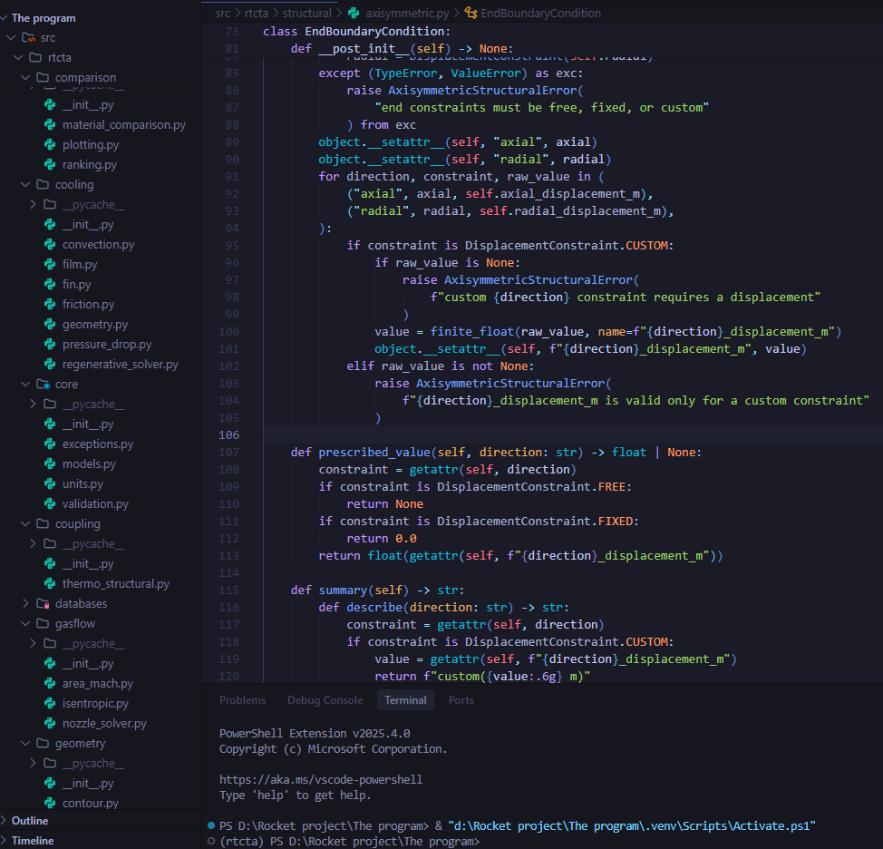
Source code of the Rocket Thrust Chamber Thermal Analysis program.

Figure 5. Source code of Rocket Thrust Chamber Thermal Analysis (RTCTA) I created myself.

Here is some results I got for the rocket performance.

Imported axisymmetric x-r contour used by the in-house rocket-thrust-chamber analysis program.

Quasi-one-dimensional gas-state and wall-boundary results from the in-house program.

Regenerative coolant state along the thrust chamber from the in-house program.

Thermal state by material along the thrust chamber from the in-house program.

Heat flux and heat-transfer coefficient along the thrust chamber from the in-house program.

Pressure march through the thrust chamber and regenerative cooling channel.

Global thermo-mechanical result from the in-house program.

Global axisymmetric and local cooling-channel thermo-mechanical results from the in-house program.

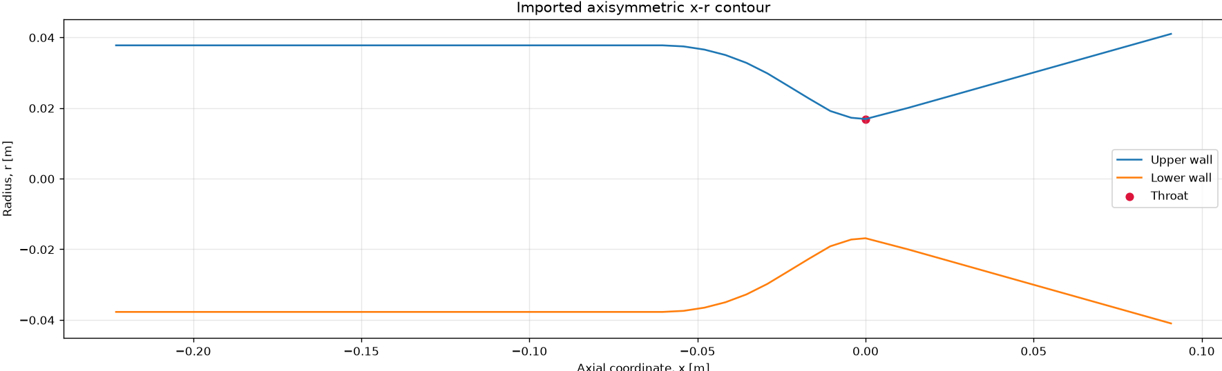
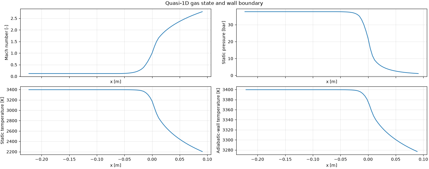
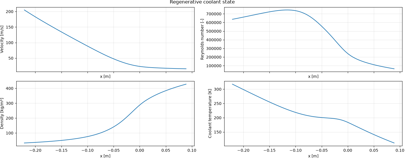
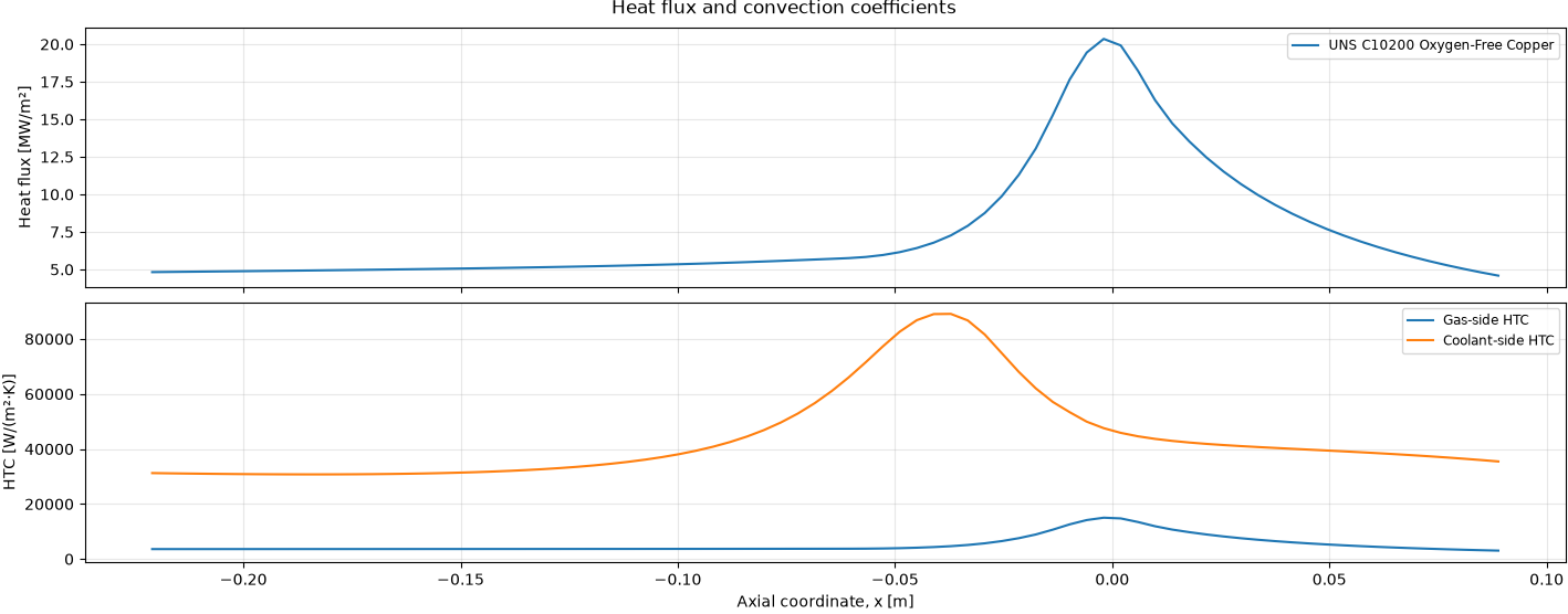
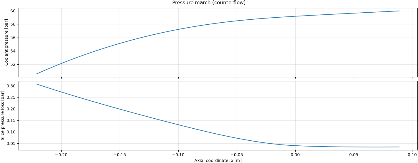
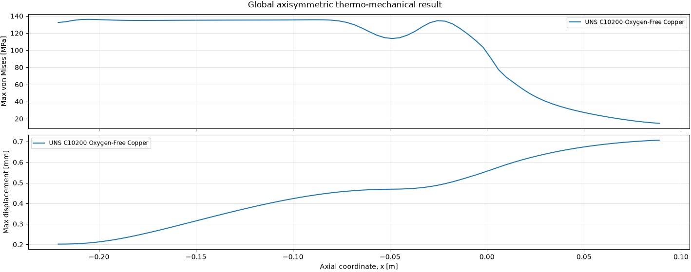
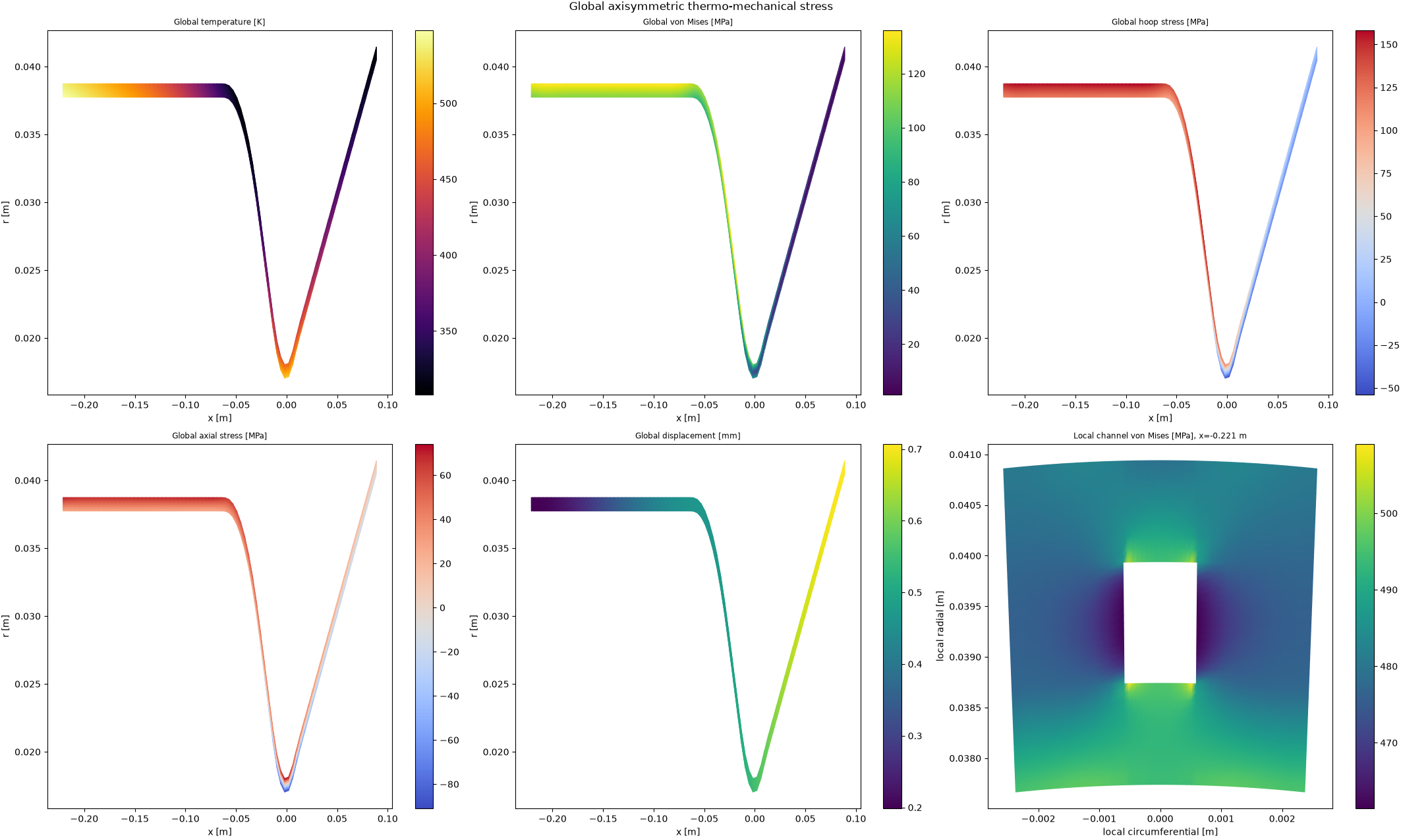
Figure 6. The result of the program, this is useful for preliminary result and for fast iteration design.

As you can see from the result, one of the highest von misses stress is around 150MPa which is still safe for selected material C10200. The pressure drop along the regenerative cooling channel is around 9.5 bars, from 60 bars to 50.5 bars which categorized as a good result because the methane is still in the supercritical regime. Minimum yield safety factor is located at -0.2 with 0.2. This small value is reasonable because that location is close to the support, which hold the highest hoop stress, axial stress, and has the minimum displacement.

\mathrm{Safety\ Factor}=\frac{\sigma_{\mathrm{yield}}}{\sigma_{\max}}

That’s why, If I only use 1mm inner wall thickness and 1 mm outer wall thickness, with 3.2 mm total chamber thickness, the rocket would absolutely explode. That’s why, in the 3D CAD, I make the thickness around this area larger. In the local channel von misses criteria, we can see that the stress is localized, concentrated at the upper and lower (inner and outer) wall of the channel with the highest value sit at around 300 MPa. This is make sense because of the pressure difference between the environment, cooling channel, and the thrust chamber itself.

I use methane for the regenerative cooler. Before methane is injected into the combustion chamber, it would flow through the engine downstream manifold, flow to the regenerative cooling channel, and then enter the upstream manifold before being injected through the injector. I use compressed liquid methane with 6 MPa at 110 K when it enters the downstream manifold and 240 K, 5.05 MPa when it enters the fuel manifold. The usage of cryogenic methane is reasonable because the engine produces 3300K adiabatic flame temperature and 3.8Mpa in the combustion chamber; it’s clear no materials could withstand these conditions. Regenerative cooling is needed.

After I got the geometry, the wall thickness, the regenerative cooling tube geometry, etc. I started to make the 3D model in SolidWorks. This is how the rocket engine looks with 19 injectors in it (I’ll discuss the injector design in a separate session).

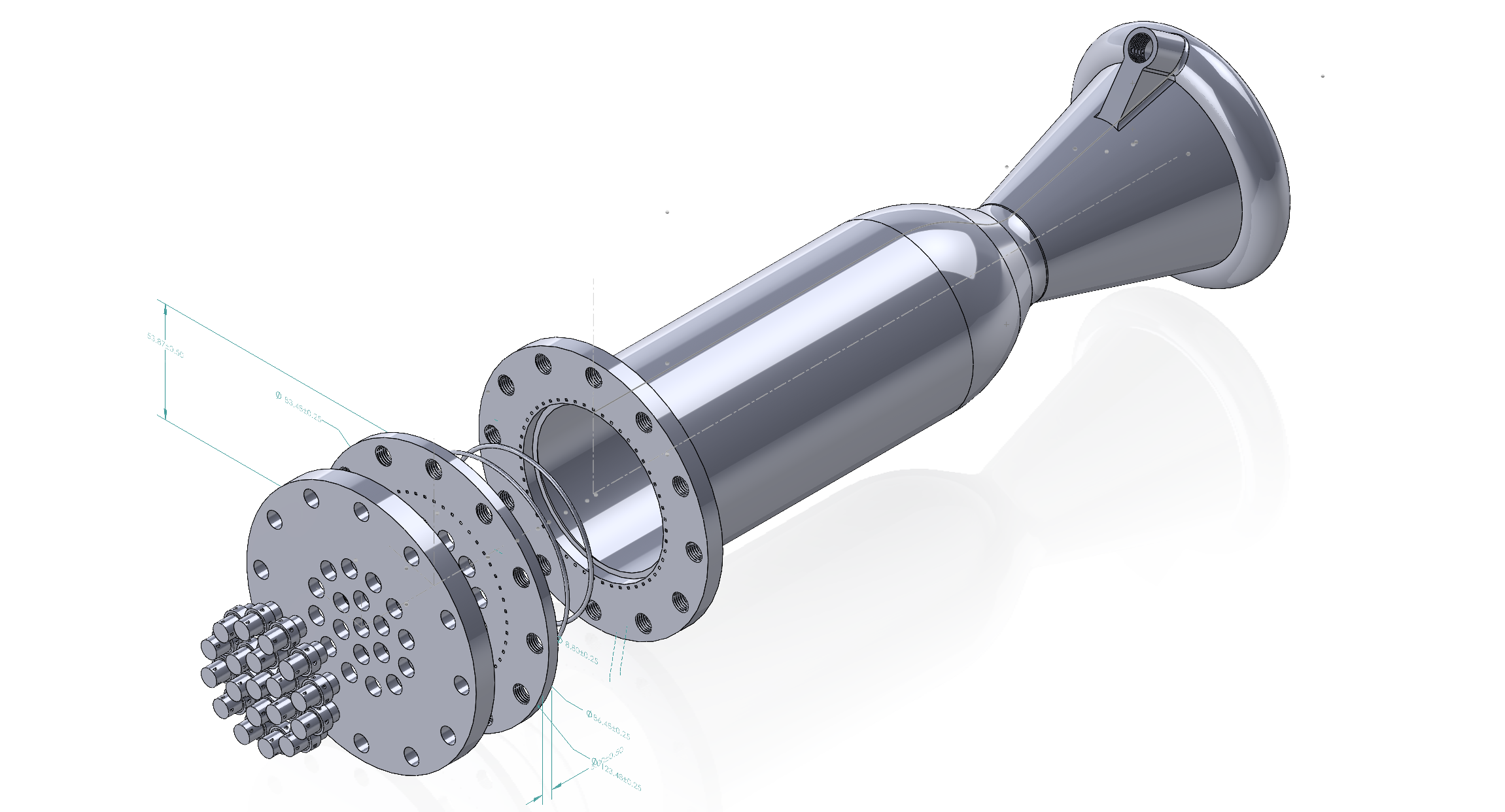
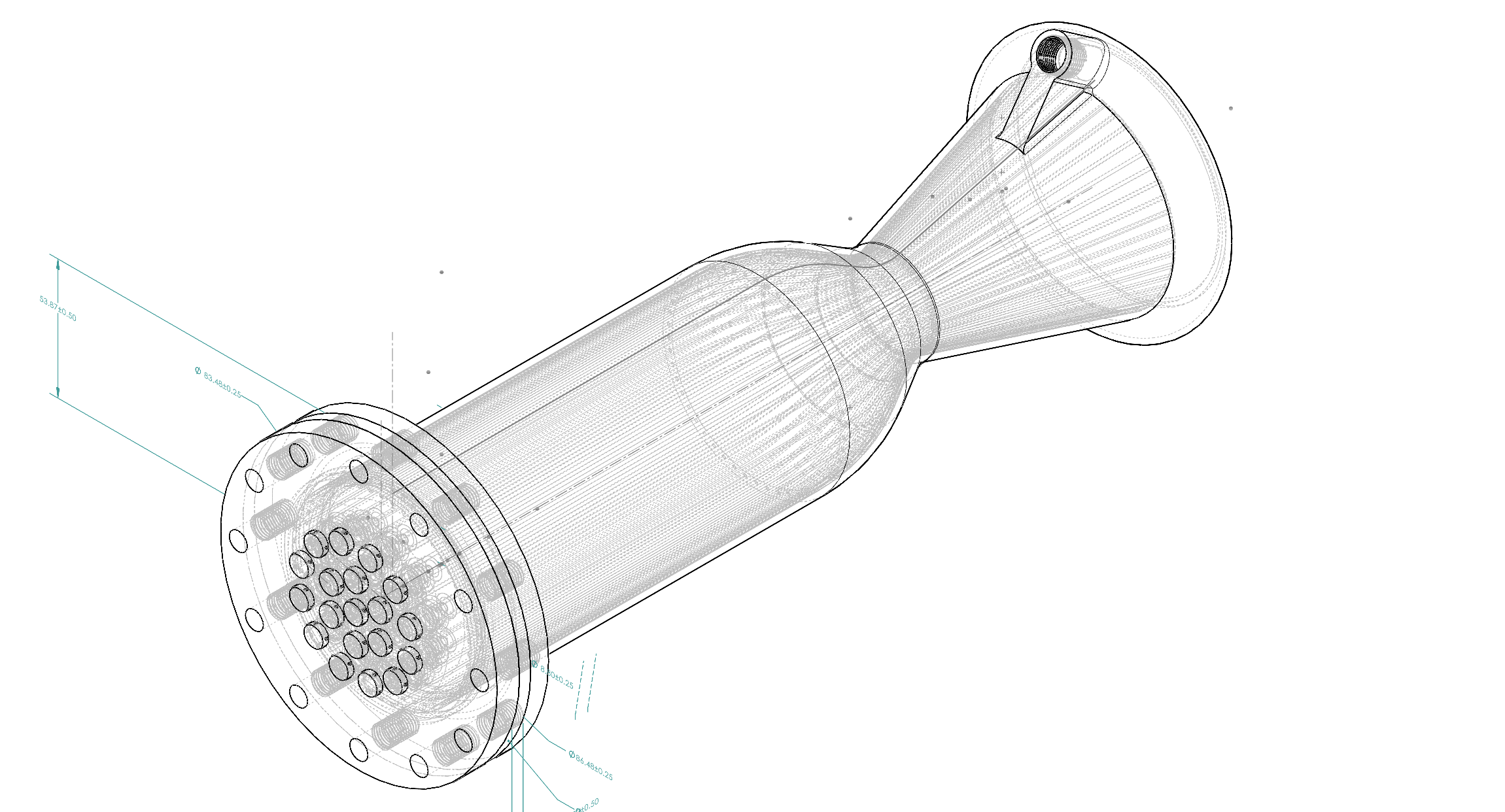
Exploded CAD assembly of the 5 kN methalox rocket engine with the injector elements, plates, chamber, manifolds, and nozzle separated.

Wireframe view of the assembled 5 kN methalox rocket engine and its internal injector and cooling geometry.

Figure 7. Exploded view and the assembly wireframe of the rocket engine.

CFD and Thermal-Mechanical Simulation

And finally, it’s time to simulate our rocket. Here, I use ANSYS Fluent and structural to simulate the CFD and thermal-mechanical stress.

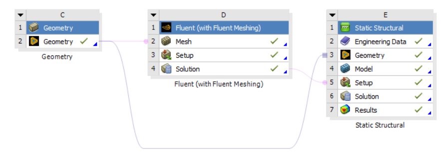
ANSYS Fluent and Static Structural workflow used for the coupled rocket-engine simulation.

Figure 8. The ANSYS Fluent-Structural setup.

I use conjugate heat transfer (CHT) simulation here coupled with thermal-mechanical structural analysis. Here is some result of this coupled simulation.

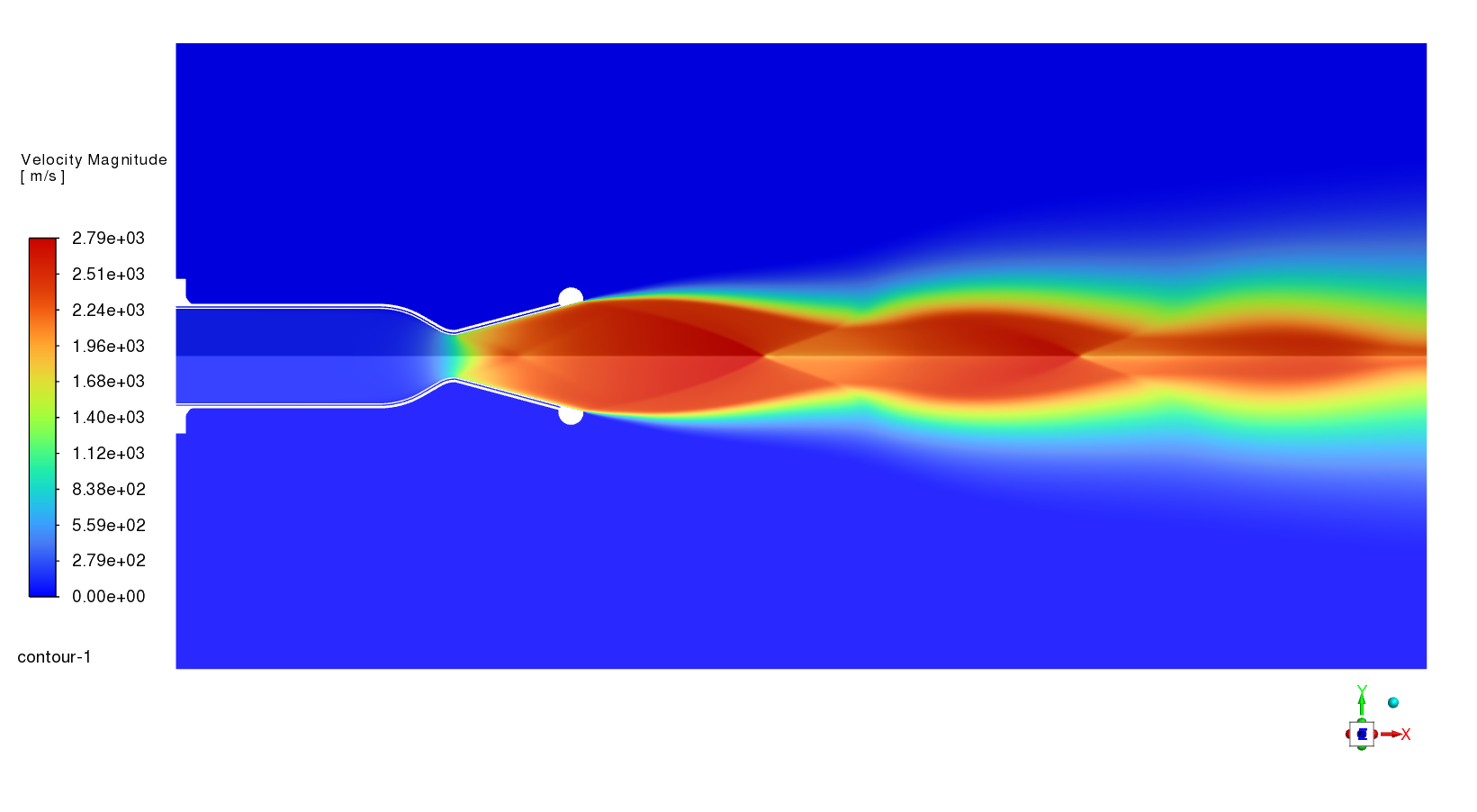
Velocity-magnitude contour through the combustion chamber and nozzle.

Figure 9. Velocity magnitude

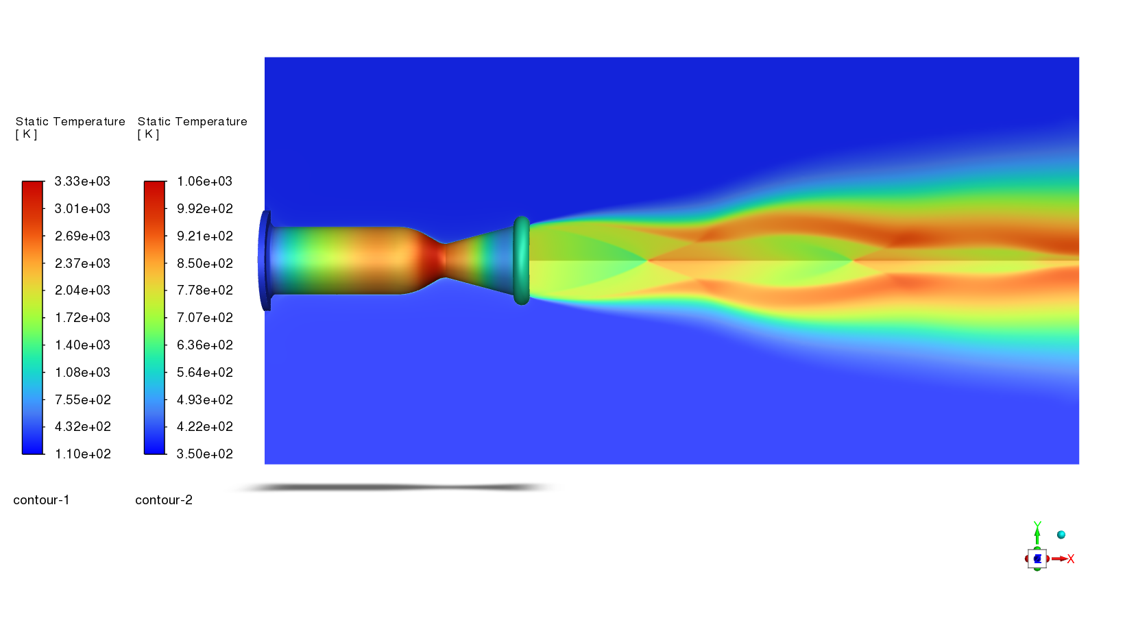
Static-temperature contour for the combustion gas and thrust-chamber wall.

Figure 10. Static temperature for the gas and wall thrust chamber

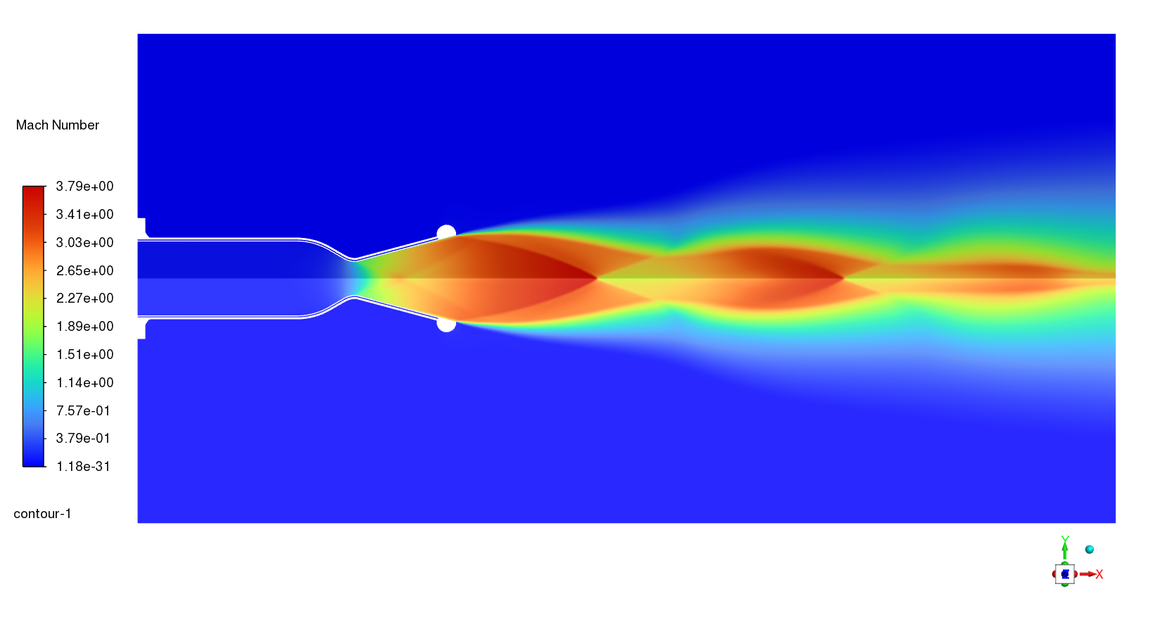
Mach-number contour through the combustion chamber and nozzle.

Figure 11. Mach number.

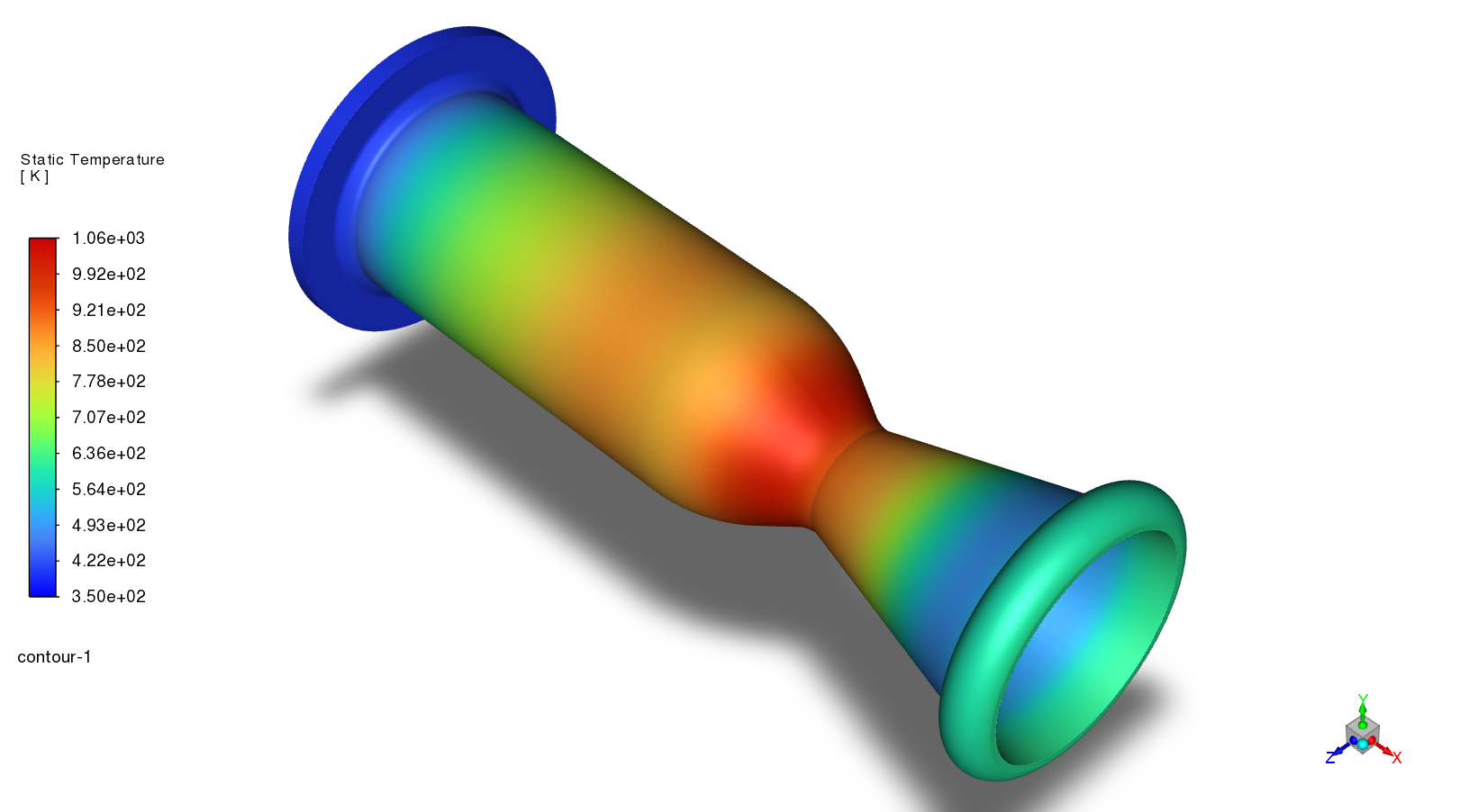
Static-temperature contour of the thrust-chamber wall.

Figure 12. Wall thrust chamber static temperature.

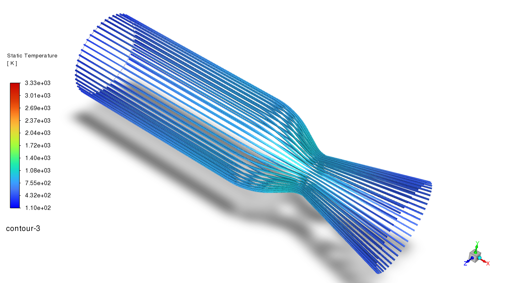
Temperature contour and coolant-flow path through the regenerative cooling channel.

Figure 13. Regenerative cooling channel temperature along the thrust chamber.

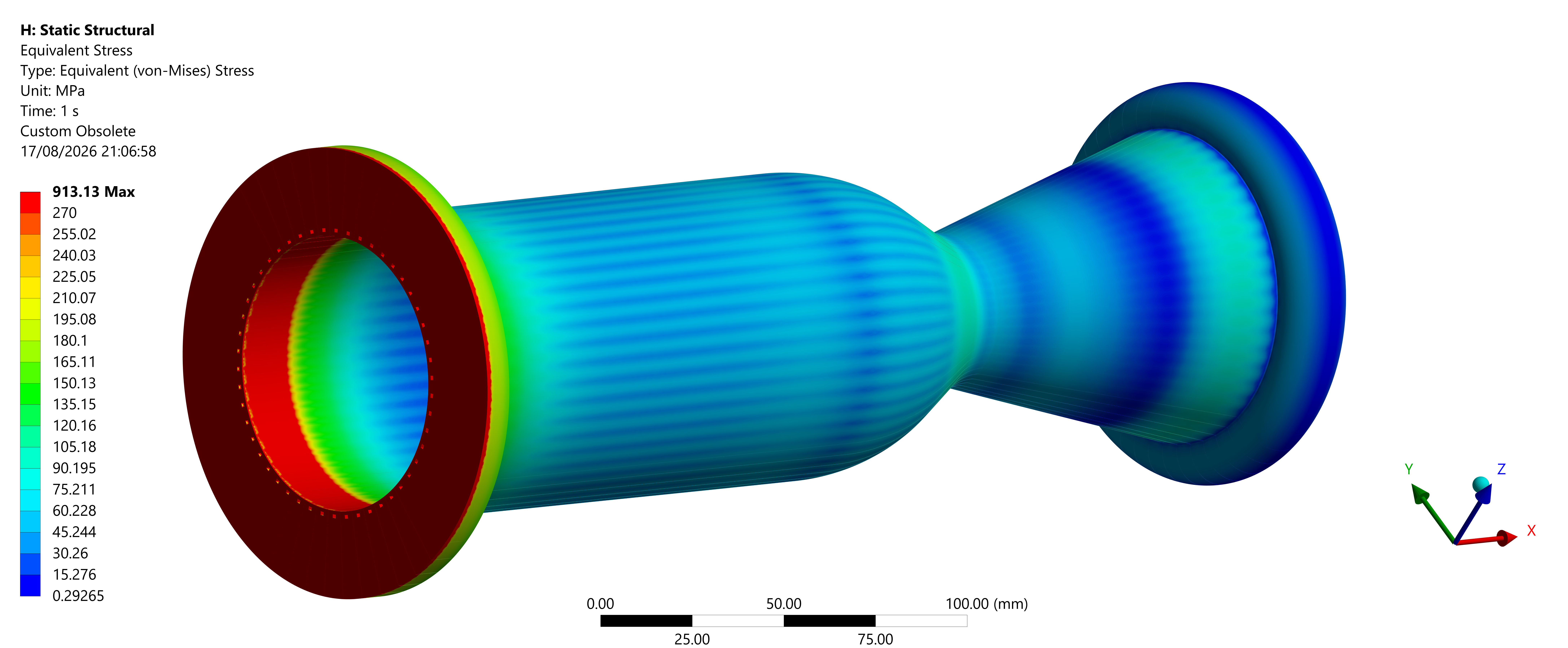
Static structural equivalent von Mises stress across the rocket-engine assembly.

Figure 14. Static structural equivalent (Von-Misses) stress

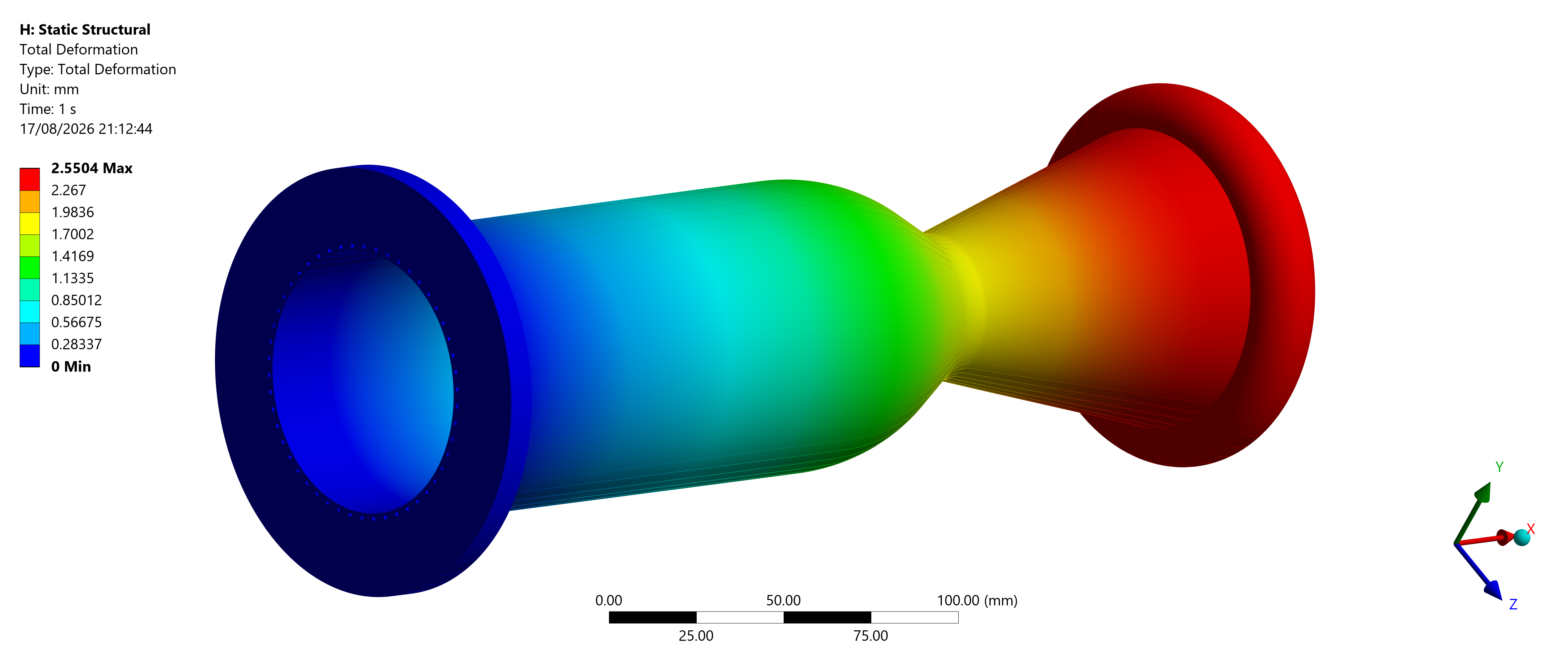
Total deformation across the complete rocket-engine assembly.

Figure 15. Total deformation

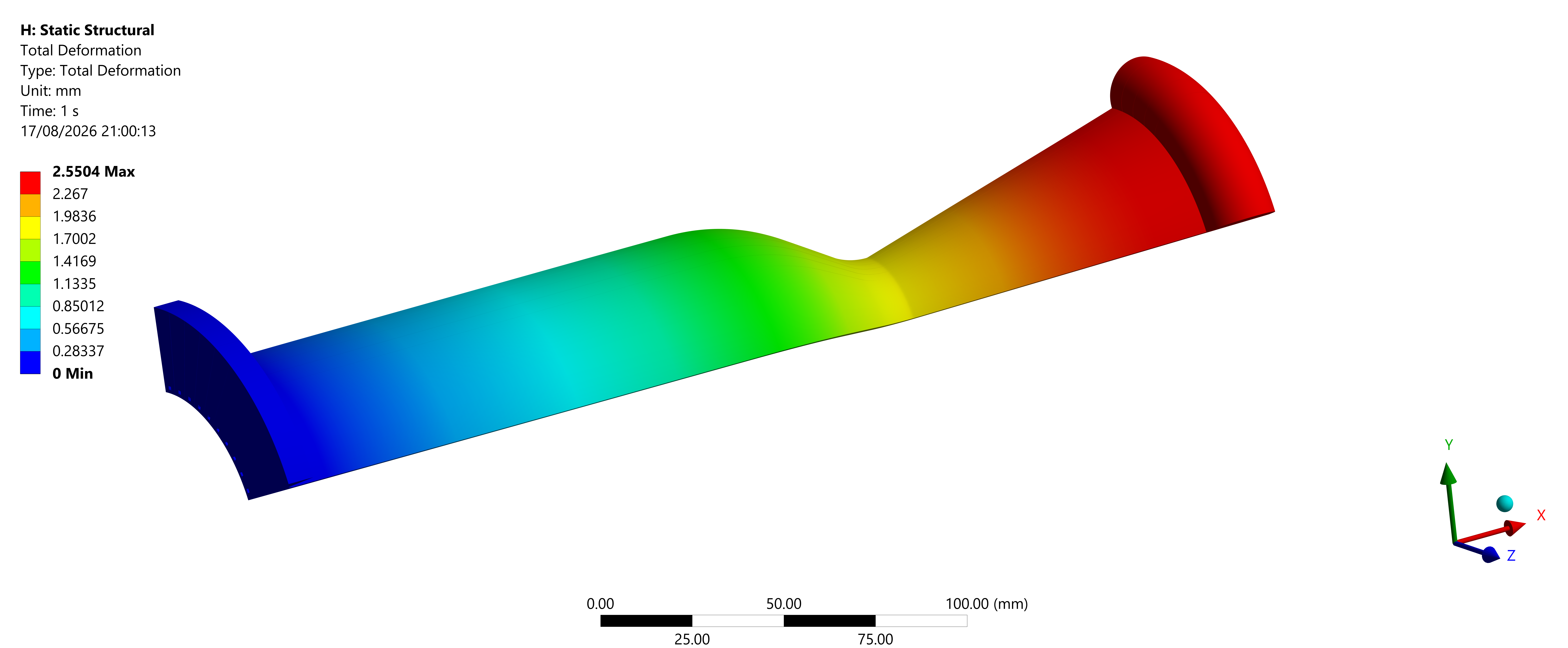
Sliced total-deformation result through the thrust chamber and nozzle.

Figure 16. Sliced total deformation.

As we can see, the result from the coupled CFD-structural simulation has some significant discrepancies. Some noticeable distinctions here are: The wall maximum temperature and the location of the wall maximum temperature. The program predicts the wall maximum temperature around 530K close to the mouth of the combustion chamber, while CFD is around 1000K at the throat. This huge difference is because, in the program, I use global film cooling effectiveness from the upstream to the downstream. On the other hand, CFD calculates the complete interaction between hot gas and the film cooling. It calculates the complete mass diffusion and reaction mechanism. That’s why, close to the throat, the film cooling effectiveness significantly decreases, resulting in a high-temperature region in that area. This 1000K temperature is dangerous for the continuous operation of the rocket engine. That’s why another solution is to add a film cooling hole close to the throat to prevent heat like Figure 17. This technique is widely used in some rocket engine designs such as Raptor, Merlin, or F-1.

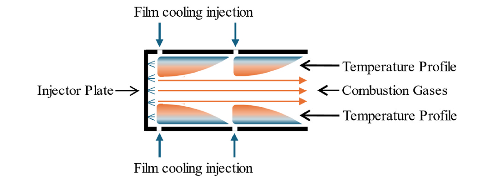
Multiple film-cooling injection concept with additional cooling holes near the throat.

Figure 17. Multiple film cooling injection.

P&ID Schematic

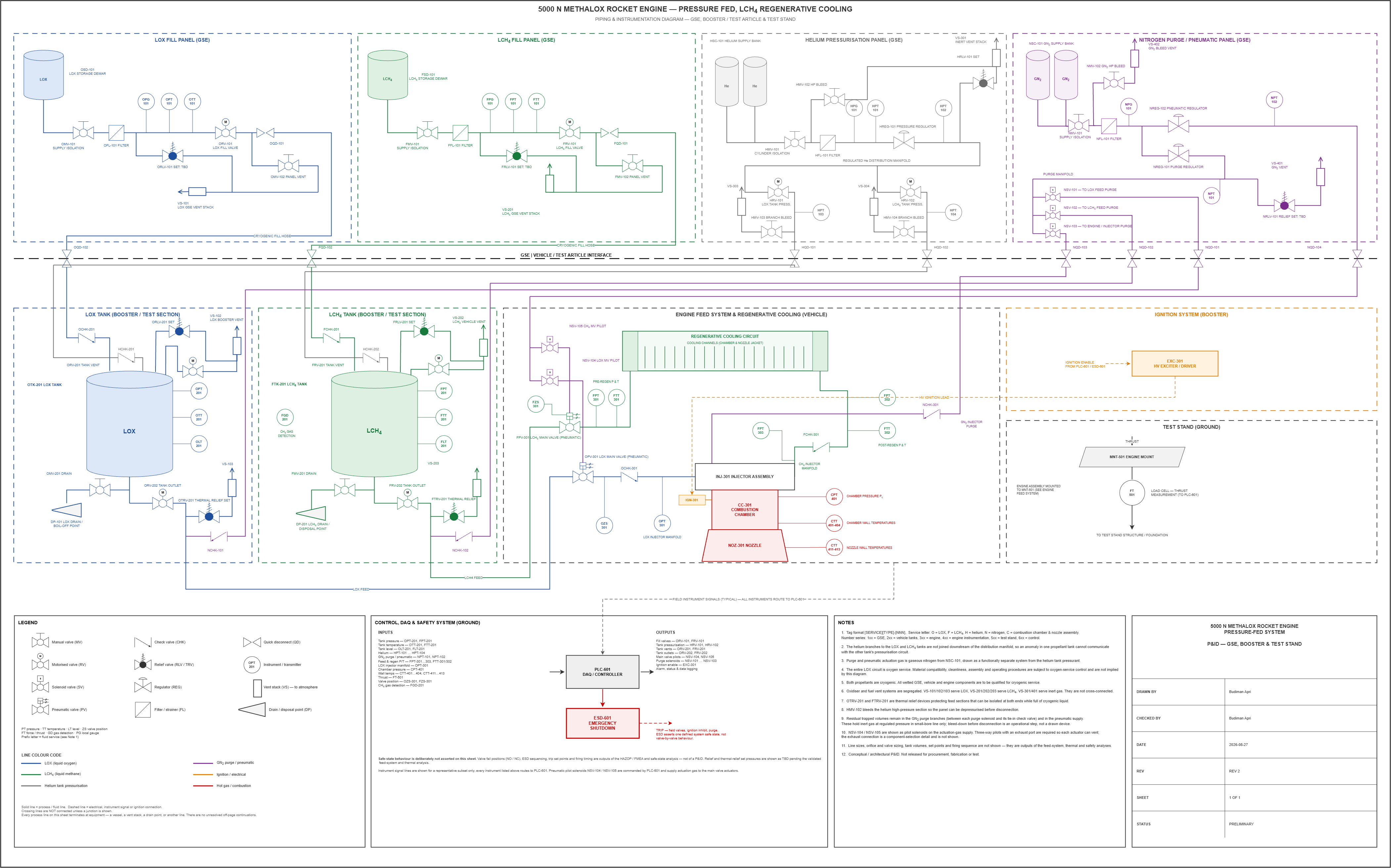
I need to fix the design further. But, to be honest, this is a promising result. Overall, my design meets the requirements. With a small adjustment, I think it can work perfectly. At the same time, I also make a piping and instrumentation diagram (P&ID) for the complete ground support, engine testbed, and all important components must be existing.

Complete piping and instrumentation diagram for the 5 kN methalox rocket engine, including ground-support fill panels, propellant tanks, helium pressurization, regenerative cooling, ignition, test stand, controls, data acquisition, and emergency shutdown — *Figure 18. Rocket piping and instrumentation diagram*

Reference

Sutton, G. P., & Ross, D. M. (1976). Rocket propulsion elements: an introduction to the engineering of rockets. Wiley.

Huzel, D. K. (1992). Modern engineering for design of liquid-propellant rocket engines (Vol. 147). AiAA.

Gândara, T., Costa, V., & Dias, J. (2025). A novel heat transfer modeling methodology for regenerative cooling in liquid propellant rocket engines. Case Studies in Thermal Engineering, 73, 106623.

D.R. Bartz, A Simple Equation for Rapid Estimation of Rocket Nozzle Convective Heat Transfer Coefficients – Technical Note DA-040495, California Institute of Technology, Pasadena, 1957.

F.M. White, Viscous Fluid Flow, McGraw-Hill, New York, 1974.

A. Alizadeh, A.M. Abed, H. Zekri, G.F. Smaisim, B. Jalili, P. Pasha, D.D. Ganji, Numerical investigation of the effect of the turbulator geometry (disturber) on heat transfer in a channel with a square section, Alex. Eng. J. 69 (2023) 383–402, https://doi.org/10.1016/j.aej.2023.02.003.

T. Kanda, M. Sato, Radiative heating in combustion chamber of liquid propellant rocket engines, Trans. Jpn. Soc. Aeronaut. Space Sci. 59 (2016) 332–339, https://doi.org/10.2322/tjsass.59.332.