NH₃ H₂ N₂ Combustion Reduced Order Model

Integration of adiabatic CFD, conjugate heat-transfer simulation, Cantera/Otomo finite-rate chemistry, and experimental residual machine learning

Sectional Divisions

Here, I will explain the full pipeline: the background, how it works, the architecture, and the data used. I’ll divide this project into some sections so the reader can understand it more easily. Sections 5-10 explain the coupled CFD-CHT-chemistry-ML model. Sections 11-14 define outputs, validation, uncertainty, and limitations. The appendices provide the equation index, all mechanism species, artifacts, and reproducibility commands.

Section	Purpose
1-4	Purpose, architecture, evidence sources, operating variables and fuel chemistry
5	Adiabatic CFD response surfaces and off-design inlet correction
6	CHT extraction, heat-transfer equations, calibration and thermal march
7-8	Residence time, flame-edge state, Otomo/Cantera finite-rate chemistry
9-10	Experimental residual ML for outlet temperature and NO
11-13	Runtime outputs, validation, uncertainty, and limitations
Appendices	Symbols/equations, 32 species, references

0. Background

Imagine running every single combustion simulation or doing every experiment to get temperature or NO results. It will take more time than we can imagine. And that is what we’re experiencing. Every time we question temperature, NO, or other combustion species, the very first thing come to our mind is simulation or experiment. We can’t use plain Cantera or adiabatic 0D or 1D flame to predict our NO or temperature because this burner is constructed using quartz, a very non-adiabatic material.

I have been involved in this project for more than 3 years since I was still an undergrad student. Brief history: this project is a collaboration project between Mitsubishi Heavy Industries (MHI) and my college, ITB. In this project, our final objective is to build an experimental combustion lab and research ammonia-hydrogen-nitrogen swirling combustion. We want to know the effect of equivalence ratio, swirl number, ammonia fraction, and Reynolds number on NO production. We need to collect so much NO and temperature data with more than 2000 simulation and experimental points need to do and potentially increase to more than 10000 if we do full experimental and simulation points: 5-10 Reynolds numbers, 5 swirl numbers, 20 equivalence ratio points each, and 10 ammonia fraction variations. That’s a lot of work.

To overcome this massive amount of data, we planned to just select some important points and simulate them in CFD adiabatic conditions in the 2nd year. In the last 3 months of the same year, we also experimented, and the result shocked us because the temperature and NO values from experiments were neither close to the CFD. Or maybe the correct way to say it is: CFD adiabatic combustion failed to predict the real NO value. We’ve generated more than 800 simulations at that time, and no one is close to the experimental result. Then we decided to continue with the experimental result and stop/close the adiabatic combustion simulation.

But we haven’t given up yet with the simulation. I proposed to the team to use a conjugate heat transfer model. Finally, we tried to use conjugate heat transfer simulation (CHT), and surprisingly, the result was so good that we could even predict the lean and rich limit blow-out.

Then we tried to simulate other cases with CHT, and all agreed with the experimental result, with temperature error average 5% and NO emission error around 8-11%. However, although CHT simulation is very accurate, this kind of simulation is computationally expensive. We only could generate total of 35 CHT simulations in 2025 in total.

To overcome all of those problems and close the gap between plan and realization, in 2026 I have an idea to use physics-guided reduced-order modelling. In a simple sentence, it’s like: “Use physics to determine how the combustion system should behave, and use machine learning only to learn the discrepancy between that physics and reality”.

1. Executive summary

The project is a physics-guided reduced-order model of a single-stage premixed NH3/H2/N2 quartz-tube burner. Its purpose is to predict the outlet/probe temperature, nitrogen oxide concentration, and the full finite-rate product composition for an operating point defined by equivalence ratio, injector Reynolds label, cracked-ammonia composition, swirl number, inlet temperature, and pressure.

It is not a single black-box regressor. The production result is assembled from four connected models: an adiabatic CFD surrogate, a CHT-informed heat-loss ROM, a Cantera implementation of the 32-species/213-reaction Otomo mechanism, and experimental residual learners for temperature and NO. The physics path gives the model a response to temperature, pressure, composition, heat transfer, residence time, and element conservation. Machine learning is reserved for discrepancies that the reduced physics cannot resolve at acceptable accuracy.

Adiabatic CFD: 597 accepted CFD rows train response surfaces for the adiabatic probe temperature and adiabatic NO.
Heat-loss bridge: 15 real CHT cases identify an operating-condition-dependent effective gas-radiation closure and test transfer on withheld cases.
Chemistry: A finite-rate flame-edge state is advanced through the non-adiabatic temperature history with the Otomo mechanism, returning all 32 mole fractions.
Experimental correction: 629 temperatures train a grouped, non-leaking residual model; 623 positive NO measurements form 48 complete curves used by a regime-aware residual hybrid.
Single runtime: The GUI and command line both call PredictionEngine, preventing two different implementations from producing different values.

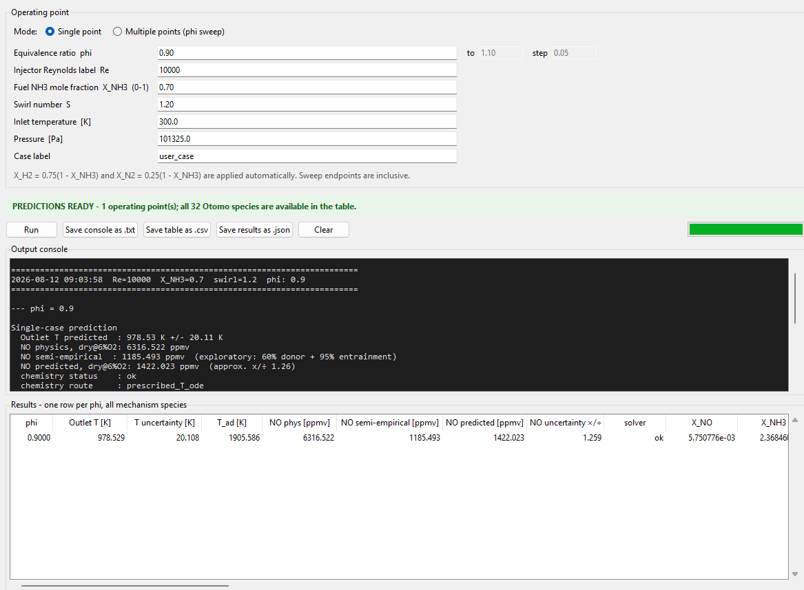
Desktop interface for entering burner operating conditions and reviewing temperature, NO, solver status, uncertainty, and the complete species output.

Figure 1. GUI of NH3-H2-N2 combustion ROM.

2. Overall architecture and information flow

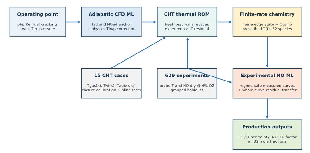
Production architecture linking the operating point, adiabatic CFD surrogate, CHT thermal ROM, finite-rate chemistry, experimental residual models, and shared outputs.

Figure 2. Production architecture. CFD, CHT, chemistry and experimental ML remain distinct but are evaluated in one ordered chain.

Figure 2 shows how the production architecture used in this project. The model first computes an adiabatic state, then predicts how the burner loses heat, then integrates chemistry along that thermal history. Only after a physics result exists does the experimental model estimate the remaining discrepancy. For temperature, the discrepancy is converted back into an effective emissivity and the thermal problem is rerun before chemistry. Consequently, the displayed temperature and the temperature seen by all species are the same physical history, not two disconnected outputs.

Layer A - adiabatic CFD surrogate: x -> Tad,CFD and NOad,CFD.
Layer B - thermal ROM: Tad -> Tgas(x), Twall,in(x), Twall,out(x), q''(x), velocity and residence-time coordinates.
Layer C - chemistry: finite-rate flame-edge composition + prescribed T(t) -> Yk(t) and outlet species.
Layer D - data discrepancy: experimental temperature and NO residual models correct the unresolved difference between reduced physics and the rig.

3. Evidence base and data governance

Table 1. Data evaluation and pre-processing.

Source	Current size	Information supplied	Role
Adiabatic CFD	869 delivered; 597 accepted	Tad probe, NO probe and available products	Surrogate training after immutable QA quarantine
Real CHT CFD	15 cases	Tgas(x), Twall,in/out(x), wall fluxes, mass flow	Thermal closure identification and blind transfer
Experiment	629 rows	629 temperatures; 625 reported NO; 623 positive targets	Temperature residual ML, NO curves and validation
Flame library	75 converged states	32-species finite-rate edge states	Chemistry initial condition over phi and XNH3
Mechanism	32 species, 213 reactions	Thermochemistry and reaction rates	Otomo/UT-LCS converted to Cantera

At this stage, I evaluate all experimental and CFD data—both adiabatic and non-adiabatic. This is a crucial step because errors in simulations or experiments that produce data outliers can cause the model to malfunction—a problem I encountered repeatedly during this process. In fact, I likely spent 20–30% of my time here simply evaluating the existing data. Outliers—such as anomalous simulation results or experimental data that deviate from expected trends (likely due to experimental error)—are excluded at this stage.

4. Operating variables, cracked-fuel family and stoichiometry

The fuel follows the ammonia-cracking identity NH3 -> 1.5 H2 + 0.5 N2, which locks H2:N2 at 3:1 in the cracked portion. The independent composition coordinate is therefore XNH3 in the fuel stream.

(1)

X_{H_2}=0.75(1-X_{NH_3}), \qquad X_{N_2}=0.25(1-X_{NH_3})

Meaning. The remaining fuel fraction after NH3 is divided into three parts H2 and one part N2 on a molar basis.

(2)

\nu_{O_2,st}=0.75X_{NH_3}+0.50X_{H_2}

Meaning. This is the stoichiometric oxygen demand per mole of the complete fuel mixture. Fuel-side N2 is inert in this oxygen balance.

How it is used. It constructs the air requirement and provides an independent cross-check of Cantera set_equivalence_ratio.

(3)

FAR_{st}=\frac{M_{fuel}}{\left(\nu_{O_2,st}/X_{O_2,air}\right)M_{air}}

Meaning. FARst is the stoichiometric mass fuel-to-air ratio, computed from the actual fuel molar mass and oxygen demand.

How it is used. The campaign equivalence ratio is mass-based over the full NH3+H2+N2 stream. FARst happens to be invariant on the 3:1 cracking line, but the code still evaluates it from composition so off-line blends are not silently mishandled.

(4)

\phi=\frac{\dot m_{fuel}/\dot m_{air}}{FAR_{st}}

Meaning. Equivalence ratio compares the actual mass fuel/air ratio to the stoichiometric ratio.

How it is used. This definition reproduces the delivered flow settings and determines the premixed Cantera inlet composition.

(5)

\dot m=\frac{Re_{label}\pi D_{inj}\mu_{mix}(T_{in})}{4}

Meaning. The workbook Reynolds number is an injector-plane label based on (D_{inj}=0.044) m.

How it is used. The equation recovers total mass flow from the label. Re_label is never used in tube heat-transfer correlations because the burner tube diameter and hot-gas viscosity differ strongly from injector conditions.

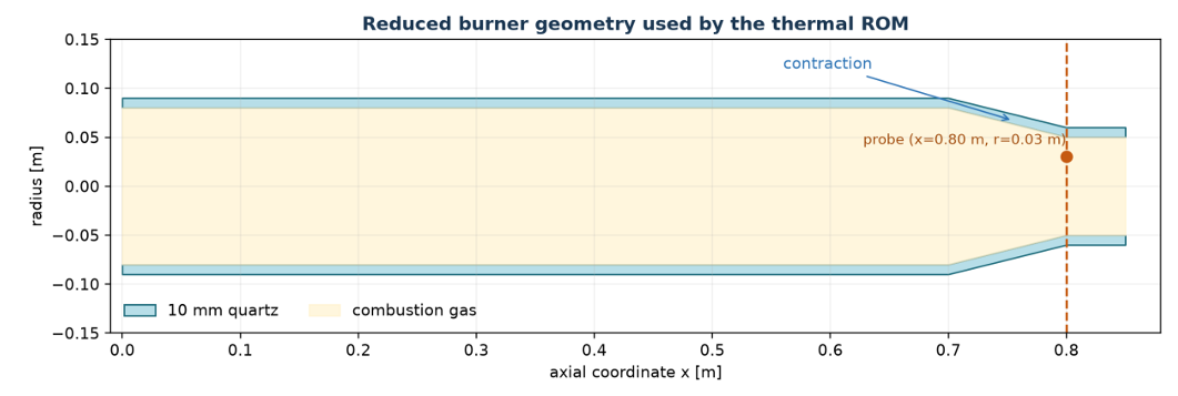
Reduced axisymmetric burner geometry showing the quartz wall, combustion-gas region, tube contraction, and off-axis probe location.

Figure 3. Piecewise axisymmetric geometry. The main tube contracts from 0.16 m to 0.10 m diameter before the off-axis probe.

5. Adiabatic CFD response surfaces

Running hundreds of CFD cases during every interactive query is impractical. Layer A replaces the accepted adiabatic CFD table with supervised response surfaces using phi, log10(Re), XNH3 and swirl as features. Inlet temperature and pressure are excluded from this fit because the CFD design contains only 300 K and 1 atm condition (no inlet pressure or temperature difference); which means, inventing learned derivatives from constant columns would be meaningless.

Target	Selected model	Fit space	GridCell CV RMSE	GridCell CV R2
Adiabatic probe temperature	Gradient boosting	identity	1.34 K	0.99997
Adiabatic probe NO	Gaussian process	log10	0.0151 dex	0.99859

From the algorithm evaluation process, I evaluate the performance of 7 surrogate models (HistGrad Boosting, Gaussian process, MLP, Ridge, Polynomial Ridge, RandomForest, Voting ensemble) by comparing the predicted values with the actual values from the CFD simulations (I only shows the best 2 here). I use the GridCell CV RMSE and GridCell CV R2 metrics to evaluate the performance of the surrogate models. I also perform leave-one-factor-level-out tests to evaluate the performance of the surrogate models under different conditions.

(6)

z_{NO}=\log_{10}(X_{NO}), \qquad X_{NO,pred}=10^{z_{NO,pred}}

Meaning. Adiabatic NO spans orders of magnitude, so the surrogate is trained in logarithmic space.

How it is used. Log-space fitting prevents high-NO cases from dominating squared error and makes multiplicative errors approximately symmetric.

5.1 Inlet temperature and pressure outside the CFD design

The CFD response surfaces alone cannot know how Tad or NO changes with inlet temperature and pressure. Production therefore computes a Cantera HP-equilibrium anchor at the query and at the CFD reference condition, then transfers only the physics-derived change onto the CFD surrogate.

(7)

T_{ad}(query)=T_{ad,CFD}(x)+\left[T_{eq,HP}(query)-T_{eq,HP}(reference)\right]

Meaning. The CFD model supplies the burner-specific baseline while equilibrium supplies the thermodynamic inlet-condition derivative.

How it is used. Changing Tin or pressure moves the upstream anchor even though those dimensions were absent from the CFD training table.

(8)

NO_{ad}(query)=NO_{ad,CFD}(x)\left[\frac{NO_{eq}(query)}{NO_{eq}(reference)}\right]

Meaning. A positive equilibrium ratio scales the adiabatic CFD NO anchor.

How it is used. This is an off-design physics correction, not a claim that the finite-rate burner is itself at equilibrium; downstream finite-rate chemistry and experimental residual correction remain active.

6. Bridging conjugate heat-transfer CFD to the thermal ROM

CHT simulations contain detailed axial and radial fields, whereas the production model needs a fast one-dimensional description. Each real CHT case is reduced to 30-60 axial stations containing mass-flow-weighted gas temperature, inner and outer wall temperature, inner total/conductive/radiative wall flux, outer wall flux, mass flow, and flame indicators. Mass-flow drift, sign convention, station ordering and the quartz conduction identity are checked before any parameter is fitted.

(9)

h_{g,eff}(x)=\frac{q''_{wall}(x)}{T_{bulk}(x)-T_{wall,in}(x)}

Meaning. This diagnostic lumps gas convection and radiation into one apparent coefficient.

How it is used. It is used to inspect CHT exports and mechanism dominance, not as the transferable closure, because convection scales linearly with temperature difference while radiation scales with the fourth power.

(10)

h_{ext,total}(x)=\frac{q''_{outer}(x)}{T_{wall,out}(x)-T_{far}}

Meaning. The external coefficient is extracted from the resolved surrounding-air CHT domain.

How it is used. The model does not pretend Fluent used an imposed external h. The extracted value is a comparison/uncertainty diagnostic for the external natural-convection plus radiation model.

(11)

q''_{cond}r_i=\frac{k_q(T_{wall,in}-T_{wall,out})}{\ln(r_o/r_i)}

Meaning. This is steady cylindrical quartz conduction on the inner-area basis.

How it is used. It is a zero-parameter export check. For semi-transparent quartz, (q”_{cond}) is the conductive component, not the total surface flux. Failure indicates wrong surfaces, units or flux decomposition and blocks fitting.

6.1 Gas-side convection

(12)

Re_D(x)=\frac{4\dot m}{\pi D(x)\mu(T,x)}

Meaning. The local tube Reynolds number changes with contraction and hot-gas viscosity.

How it is used. It selects laminar, transition or turbulent heat-transfer behavior at every axial station. The observed range is approximately 1400-5500, so Dittus-Boelter is intentionally rejected.

(13)

Nu_H=3.66+\frac{0.0668Gz}{1+0.04Gz^{2/3}}, \qquad Gz=\left(\frac{D}{x}\right)RePr

Meaning. The Hausen expression adds thermal entrance effects to fully developed laminar flow.

How it is used. The main tube has L/D about 5.3, so the entrance region is not negligible. Between Re=2300 and 4000, a smoothstep blends this result with Gnielinski.

(14)

f=(0.79\ln Re-1.64)^{-2}

Nu_G= \frac{(f/8)(Re-1000)Pr} {1+12.7(f/8)^{1/2}(Pr^{2/3}-1)}

Meaning. Petukhov friction and Gnielinski heat transfer describe the turbulent-side limit.

How it is used. They act only in the declared transition/turbulent range; the code records which regime was used at each station.

(15)

h_{conv}(x)=\frac{Nu(x)k_{gas}(T,Y)}{D(x)}

Meaning. Cantera supplies temperature- and composition-dependent gas conductivity and viscosity.

How it is used. This gives only the convective inner-wall term; gas radiation remains separate.

6.2 Radiation, wall conduction and external loss

(16)

q''_{in}=h_{conv}(T_g-T_{wi})+\epsilon_{gas}\sigma(T_g^4-T_{wi}^4)

Meaning. The inner heat flux is explicitly the sum of convection and grey-gas radiation.

How it is used. Separating the two terms avoids fitting one coefficient that may interpolate the CHT cases but extrapolate incorrectly as temperature changes.

(17)

\epsilon_{gas,local} = \operatorname{clip} \left[ \epsilon_{gas,ref} \frac{X_{H_2O}}{X_{H_2O,ref}} \right]

Meaning. The effective grey-gas emissivity scales approximately with water partial amount and is bounded to a physical interval.

How it is used. The CHT-calibrated reference emissivity is adapted to the local product composition without allowing negative or greater-than-unity values.

(18)

R_{cond}=\frac{r_i\ln(r_o/r_i)}{k_q}

Meaning. Rcond is the cylindrical lattice resistance referred to the inner surface area.

How it is used. With 10 mm fused silica and (k_q=1.3787) W/m-K, the wall temperature drop is too large to justify an isothermal-wall approximation.

(19)

Nu_{ext} = \left\{ 0.60+ \frac{0.387Ra^{1/6}} {\left[1+(0.559/Pr)^{9/16}\right]^{8/27}} \right\}^2

Meaning. Churchill-Chu models natural convection from the outer horizontal cylinder.

How it is used. It supplies the modeled convective share of the external loss. External radiation remains nonlinear: (\epsilon_{wall}\sigma(T_{wo}^4-T_{sur}^4)).

The quartz in Fluent is a semi-transparent participating medium with absorption coefficient 400 1/m, refractive index 1.5 and 10 mm thickness. Its optical thickness is about 4, so the ROM uses a calibrated grey-opaque equivalent while preserving conductive and radiative heat transport in parallel. The effective wall emissivity is fixed at 0.90; epsgas is the main CHT-identified closure.

6.3 Axial energy march

(20)

h_{i+1} = h_i - \frac{\left[q''_iP_i+q''_{i+1}P_{i+1}\right]\Delta x}{2\dot m}

Meaning. A second-order Heun/trapezoidal update removes heat from the flowing gas according to the wetted perimeter.

How it is used. The ROM marches specific enthalpy, not (c_p\Delta T). Cantera inverts (h(T,Y)) with HPY, preserving variable heat capacity and the chosen composition.

(21)

\dot m\left[h_{in}-h_{out}\right] = \int q''(x)P(x)\,dx

Meaning. This is the global steady energy balance.

How it is used. Every thermal solution reports the relative closure residual and checks monotonic cooling and the ordering (T_{wo}\le T_{wi}\le T_g) whenever heat leaves the gas.

6.4 CHT calibration and transfer

Independent single-case fits identify effective epsgas at five phi levels. A shape-preserving PCHIP surface connects those nodes, while ten remaining CHT cases test transfer. This retains a small, interpretable closure rather than allowing a flexible neural network to absorb missing heat-transfer physics.

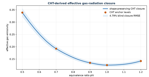
Effective gas-emissivity closure versus equivalence ratio, with CHT anchor levels and the blind-transfer uncertainty band.

Figure 4. CHT-only effective gas-emissivity surface. The shaded band shows the 4.79% relative blind closure RMSE used as a transfer uncertainty scale.

(22)

\mathbf r= \left[ \frac{T_{g,ROM}-T_{g,CHT}}{\sigma_T}, \frac{T_{wi,ROM}-T_{wi,CHT}}{\sigma_T}, \frac{q_{ROM}-q_{CHT}}{\sigma_q}, \frac{T_{probe,ROM}-T_{probe,CHT}}{\sigma_T} \right]

Meaning. Calibration minimizes normalized profile, wall-flux and probe residuals, with station-count normalization so dense files do not dominate.

How it is used. Bounded multi-start least squares fits no more than two active parameters and checks the Jacobian condition number before accepting the result.

7. Flame position and residence time

To correctly predict the finite-rate post-flame chemistry, I try to define the flame front by the gradient of the temperature in the CHT results. I choose the temperature gradient because it is a good indicator of where the flame is located. Other possible indicators such as heat-release, progress-variable and radical indicators give similar results for xflame. Current real exports do not contain a solved mean-age user-defined scalar, so production uses the declared integral one-dimensional fallback. This is because the chemistry must begin at the flame, not at the injector.

(23)

\tau_{int} = \int_{x_{flame}}^{x_{probe}}\frac{dx}{u(x)}, \qquad u(x)=\frac{\dot m}{\rho(x)A(x)}

Meaning. The parcel time is integrated through the changing density and contracted area.

How it is used. The CHT cases establish the ratio between this integral and a characteristic L/U time. The mean (C_\tau) used by runtime is approximately 1.316.

(24)

\tau_{chem}=C_\tau\tau_{int}, \qquad t_{chem}(x)=\tau_{age}(x)-\tau_{age}(x_{flame})

Meaning. Ctau accounts for unresolved recirculation/mixing relative to the one-dimensional path.

How it is used. The chemical clock is zeroed at the flame and scales the PCHIP temperature history supplied to the stiff kinetic integrator.

8. Cantera/Otomo finite-rate chemistry

First, I converted the UT-LCS/Otomo Chemkin mechanism to Cantera YAML, asserting it to contain exactly 32 species and 213 reactions. Thermodynamic and kinetic evaluation, mixture transport for flame checks, equilibrium anchors, free-flame calculations and stiff post-flame integration all use this mechanism.

8.1 Finite-rate flame-edge initial state

Starting post-flame kinetics from thermodynamic equilibrium is problematic: it leaks equilibrium NO concentrations into a process meant to predict finite-rate NO formation. To avoid this, I build a 75-state free-flame library (assuming unity Lewis number) pre-computed across equivalence ratio ( $\phi$ ) and ammonia fraction ( $X_{\text{NH}_3}$ ). I sample each flame state at the point where cumulative heat release reaches 99.5%, preserving active radical pools and incomplete reaction intermediates.

When a query falls within the library domain, I interpolate all species mole fractions across the grid. Outside the domain, I hold the radical and trace species from the nearest boundary state constant, adjusting only major stable reservoirs ( $\text{N}_2$ , $\text{H}_2\text{O}$ , $\text{O}_2$ , $\text{H}_2$ , and $\text{NH}_3$ ) to satisfy exact mass and element ( $\text{H}/\text{N}/\text{O}$ ) conservation. This approach completely eliminates artificial, discontinuous jumps to equilibrium at parameter boundaries.

(25)

\min \left\|Y-Y_{interp}\right\|_2 \quad \text{subject to} \quad AY=b_{query}, \qquad Y\ge0

Meaning. A contains total mass and elemental H/N/O mass fractions; bquery comes from the exact inlet mixture.

How it is used. The active-set projection changes stable reservoirs while preserving radical structure, and it is rejected if the maximum constraint error exceeds (1\times10^{-8}).

8.2 Prescribed-temperature kinetic integration

(26)

\frac{dY_k}{dt} = \frac{W_k\omega_k(T(t),p,Y)}{\rho}

Meaning. Cantera provides net molar production rate omega, molecular weight W and density for each species.

How it is used. A BDF stiff solver advances all species along the thermal-ROM temperature history. Negative species, mass-fraction drift, non-finite output and excessive runtime are explicit statuses, not silently clipped results.

A second constant-pressure Cantera reactor route reimposes temperature at each step as a cross-check. Across 20 comparison cases, both routes solved; the p95 absolute NO difference was 0.00594 dex, the maximum was 0.02383 dex, and elemental errors remained below about 1e-13. The prescribed-T ODE is retained as the production route because it is direct and efficient.

8.3 Mechanism validation

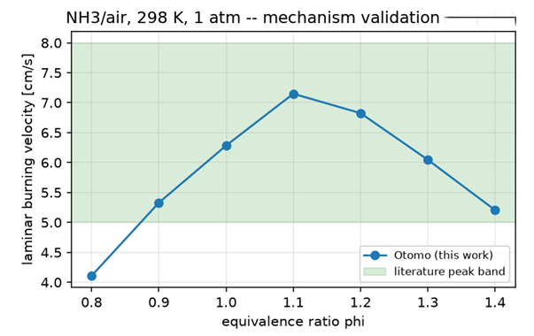
Laminar burning velocity across equivalence ratio for the Otomo ammonia-air mechanism, compared with the configured literature band.

Figure 5. Otomo NH3/air laminar flame-speed check at 298 K and 1 atm. The 7.15 cm/s peak lies in the configured 5-8 cm/s reference band.

Thanks to God, the mechanism also passes the required monotonic increase of flame speed with cracking fraction (I spent so much time here). As we can see in Figure 5, the free-flame library is rectangular and converged, all interpolated states are non-negative after projection, maximum element error is 8.66e-9, and the finite-rate edge temperature spans approximately 1431-2104 K. I found here that the maximum laminar burning velocity is at phi = 1.1, which matches the typical value for NH3/air mixture. [Gong, Xue, et al. 2026]

9. Experimental residual ML for outlet temperature

The CHT thermal ROM captures the heat-loss mechanism but leaves systematic experiment-to-ROM discrepancy. The production learner targets only that residual to compensate for the discrepancy at the next step:

(27)

\Delta T_{ML} = T_{exp,probe} - T_{physics,probe}, \qquad T_{target} = T_{physics,probe} + f_{ET}(x)

Meaning. An ExtraTrees ensemble learns the experimental discrepancy around the CHT physics baseline.

How it is used. Features are phi, log10(Re), XNH3, swirl, Tad and the physics probe temperature. The constant experimental inlet temperature and pressure are not learnable derivatives; their response continues to come from physics.

A checkerboard grouped fold assigns operating cells deterministically. Fold 0 (121 rows) is never seen by the validation estimator. After validation, the final 600-tree ExtraTrees model is fit to all eligible temperatures for production.

(28)

\epsilon_{gas}^{*} = \arg\min_{\epsilon} \left| T_{probe,ROM}(\epsilon)-T_{target} \right|

Meaning. The corrected target is inverted through the bounded thermal ROM.

How it is used. The complete thermal profile is rerun at epsgas*, then chemistry uses that profile. This prevents a post-hoc temperature overwrite from becoming inconsistent with species predictions.

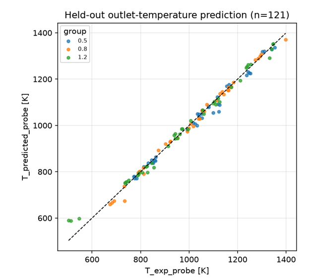
Parity plot comparing grouped-holdout predicted and experimental thermocouple outlet temperatures for 121 cases.

Figure 6. Grouped holdout parity for thermocouple-indicated outlet temperature (n=121).

Temperature metric	Result	Interpretation
RMSE	20.11 K	pass vs 40 K
Bias	-2.11 K	pass vs +/-15 K
Median absolute relative error	0.99%	descriptive
P90 absolute relative error	2.40%	descriptive
Maximum absolute relative error	17.2%	marginal vs 15% target
R2	0.9897	descriptive

Runtime uncertainty is the larger of ensemble tree spread and the 20.11 K holdout RMSE. Residual trends with Reynolds number and swirl remain statistically significant; therefore the temperature model is good.

10. Experimental residual ML for NO

NO(phi) is not a single smooth universal curve. Here, I used the experimental data to correct the NO prediction. The measurements contain abrupt lean- and rich-side transitions, and the curve shape changes with Re, cracking fraction and swirl. At the first time, my model scored only stable/interior points and then returned a broad plateau on the tails, which makes no sense. So I used a correction method to fix it and it works well. The current hybrid separates known-curve interpolation from genuine transfer to an unseen operating curve.

(29)

c_{NO} = \log_{10}(NO_{measured}) - \log_{10}(NO_{physics})

\log_{10}(NO_{pred}) = \log_{10}(NO_{physics}) + c_{NO}

Meaning. The ML target is a multiplicative correction to finite-rate physics.

How it is used. This retains physical sensitivity to temperature, pressure, residence time and chemistry while allowing the data to correct systematic NO magnitude and shape error.

10.1 Known measured curve

I group each curve by Reynolds number ( $Re$ ), ammonia fraction ( $X_{\text{NH}3}$ ), and swirl ratio. If adjacent data points show a sudden jump in NO concentration—specifically over $0.30\text{ dex}$ on a $\log{10}$ scale—I split the curve into separate segments so interpolation never blurs distinct physical regimes.

Within any continuous segment, I use PCHIP interpolation when I have at least three points, and fall back to simple linear interpolation for two-point runs. No interpolator is allowed to cross a detected regime break.

To validate this setup, I use a strict leave-one-out approach: I remove the target point before re-detecting regime breaks so the held-out value cannot influence its own segment boundary. Finally, I disclose exact campaign nodes as fixed measurement anchors rather than model predictions.

10.2 Entirely new operating curve

When predicting a curve that wasn’t included in the experimental campaign, I use a 500-tree ExtraTrees model to estimate the discrepancy ratio, $\log_{10}(\text{NO}{\text{measured}} / \text{NO}{\text{physics}})$ . The model takes seven key input features: equivalence ratio ( $\phi$ ), $\log_{10}(Re)$ , hydrogen fraction ( $X_{\text{H}2}$ ), swirl ratio, $\log{10}(\text{NO}{\text{physics}}$ ), normalized ROM temperature ( $T{\text{ROM}}/1000$ ), and residence time scale $\log_{10}(\tau)$ .

To test how well the model generalizes to unseen operating conditions, I validate it using a leave-one-whole-curve-out scheme, withholding each of the 48 operating curves in turn. When making predictions outside the domain of observed experimental data, I expand the uncertainty bounds using a normalized nearest-neighbor covering radius and factor limits, ensuring out-of-distribution uncertainty is reflected without clipping or suppressing the underlying numerical result.

(30)

\sigma_{\log NO} = \max(\text{tree spread}, RMSE_{LOCO}), \qquad \text{uncertainty factor} = 10^{\sigma_{\log NO}}

Meaning. Log uncertainty becomes an approximate multiply/divide factor in concentration space.

How it is used. Known-run interpolation uses 0.0744 dex; whole-curve transfer uses at least 0.2871 dex and uses the p90 absolute log error outside support.

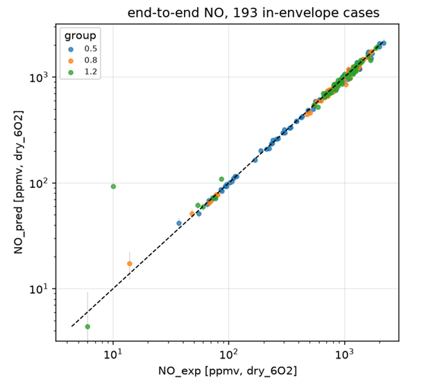
Log-scale parity plot comparing predicted and experimental NO for strict known-curve validation on a dry six-percent oxygen basis.

Figure 7. Strict known-curve NO validation on the dry, 6% O2 basis (n=193).

Validation question	n	Within +/-30% or 20 ppm	log10 RMSE	Runtime meaning
Known curve, held-out node	193	99.5%	0.0744 dex	validated interpolation
New curve, all nodes withheld	612	79.7%	0.2871 dex	best estimate; transfer gate marginal

Important distinction. The 99.5% accuracy rate applies specifically to interpolating a new equivalence ratio ( $\phi$ ) along an already measured operating curve. When evaluating an entirely new operating curve, performance drops to 79.7% within tolerance with an RMSE of $0.287\text{ dex}$ . While the model evaluates both scenarios, they carry fundamentally different uncertainty profiles and scientific confidence.

11. Product basis, complete species vector and outputs

While Cantera calculates wet mole fractions for all mechanism species, both the experimental measurements and CFD benchmark data are already reported on a dry basis and corrected to $6\%\text{ O}_2$ . Therefore, I only convert the model’s raw predictions to match this standard; I never apply a second correction to the experimental or CFD data.

(31)

X_{NO,dry} = \frac{X_{NO,wet}}{1-X_{H_2O}}

Meaning. Removing water converts wet mole fraction to a dry basis.

How it is used. The same operation gives predicted dry O2 for the oxygen-reference correction.

(32)

NO@O2_{ref} = NO_{dry} \frac{21-O2_{ref}}{21-O2_{dry}}

Meaning. This standard correction reports the concentration at 6% dry O2.

How it is used. The denominator is guarded against O2 approaching 21%, where the correction becomes singular and indicates a near-unfired condition.

12. Production prediction algorithm

Validate the numerical inputs and generate XH2 and XN2 from XNH3.
Evaluate the CFD Tad and NOad surrogates; apply Cantera HP inlet-temperature/pressure deltas.
Evaluate the CHT epsgas(phi) closure and the baseline thermal probe temperature.
Apply the experimental temperature residual model, invert bounded epsgas, and rerun the thermal profile.
Interpolate the finite-rate flame-edge state; if outside its rectangle, use the boundary state and enforce exact H/N/O conservation.
Build the velocity/residence-time coordinate and integrate the 32-species Otomo kinetics along T(t).
Convert physics NO to dry 6% O2 and evaluate the full-curve NO residual hybrid.
Return temperature, NO, all species, uncertainties, solver status and provenance through the shared GUI/CLI API.

This sequence is why the model remains useful when Tin or pressure changes: those changes enter thermodynamics, properties, heat transfer and kinetics before the empirical residual is applied. The data layer improves the result but does not provide unsupported temperature/pressure derivatives.

13. Validation, acceptance gates and scientific interpretation

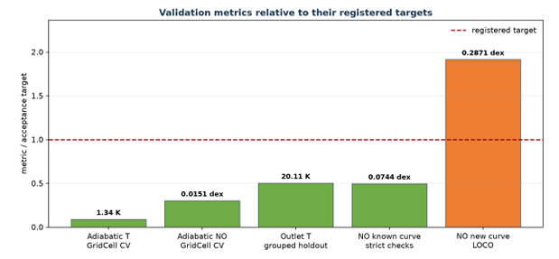
Validation metrics normalized by their registered acceptance targets, showing passing physics and known-curve metrics and a marginal new-curve NO result.

Figure 8. Major validation metrics normalized by their registered targets. Values below 1 pass; the new-curve NO log-RMSE remains marginal.

Validation layer	Status	Evidence
Data schema/definitions	pass	No silent coercion; definitions reproduce flows and locations
Adiabatic surrogates	pass	GridCell CV: 1.34 K and 0.0151 dex
CHT closure surface	pass	4.79% relative blind epsgas RMSE; worst blind probe error 24.1 K
Chemistry	pass	32/213 counts, flame-speed gate, element and mass conservation
Outlet temperature	pass/marginal	RMSE and bias pass; max 17.2%; Re/swirl residual trends remain
NO known curve	pass	99.5% within tolerance; 0.0744 dex
NO whole-curve transfer	marginal	79.7% within tolerance; 0.2871 dex

If a validation gate fails, I don’t design the software to simply refuse an answer. Instead, the model adjusts the confidence of its claim and widens the uncertainty bounds. This choice is deliberate: I believe a predictive engineering tool should always return its best physically constrained estimate, while validation flags prevent that estimate from being presented as more accurate than the evidence actually supports.

Appendix A. Equation and symbol index

Symbol	Definition	Unit
phi	equivalence ratio	-
Re_label	injector-plane Reynolds label	-
Re_D	local hot-gas tube Reynolds number	-
m_dot	total mass flow rate	kg/s
Tad	adiabatic CFD/physics anchor temperature	K
Tg	bulk gas temperature in thermal ROM	K
Twi, Two	inner and outer quartz temperatures	K
q”	inner-area heat flux, positive out of gas	W/m2
eps_gas	effective grey-gas radiation closure	-
eps_wall	grey-equivalent quartz external emissivity	-
tau_chem	post-flame chemical residence time	s
Yk, Xk	species mass and mole fractions	-
omega_k	net molar production rate	kmol/m3/s
NO@6%O2	dry NO corrected to 6% oxygen	ppmv

Equations (1)-(5) define mixture preparation and flow. Equations (6)-(8) define the adiabatic ML and off-design thermodynamic anchor. Equations (9)-(22) define CHT diagnostics, heat transfer, wall balance, energy marching and calibration. Equations (23)-(26) define residence time and chemistry. Equations (27)-(30) define the experimental residual learners and uncertainty. Equations (31)-(32) define the reporting basis.

Appendix B. Complete Otomo mechanism species

Species	Species	Species	Species
1. NO	2. NH3	3. H2	4. O2
5. H	6. O	7. OH	8. HO2
9. H2O	10. H2O2	11. NH2	12. NH
13. N	14. NNH	15. NH2OH	16. H2NO
17. HNOH	18. HNO	19. HON	20. NO2
21. HONO	22. HNO2	23. NO3	24. HONO2
25. N2O	26. N2H4	27. N2H3	28. N2H2
29. H2NN	30. AR	31. HE	32. N2

Appendix C. Sources and project references

Gong, X., Chen, X., Li, H., Pan, S., Chen, H., Bao, X., & Zhang, Z. (2026). Experimental and numerical study on laminar propagation characteristics of ammonia/air flames at elevated pressure and temperature. International Journal of Hydrogen Energy, 237, 155231.
Otomo, Koshi, Mitsumori, Iwasaki and Yamada, International Journal of Hydrogen Energy 43 (2018) 3004-3014 - kinetic mechanism source recorded in configs/cantera.yaml.
Cantera - thermodynamic properties, HP/TP equilibrium, free flames and finite-rate reaction rates.
Hausen entrance correlation; Petukhov friction factor; Gnielinski internal convection; Churchill-Chu horizontal-cylinder natural convection; Ranz-Marshall sphere heat transfer - correlations as implemented and sourced in project configuration/code.
Hayakawa et al. (2015) and Ichikawa et al. (2015) - configured NH3/air laminar-flame-speed reference band.