In part 1, I explained why radiation is so important and how it could influence the performance and structural and material selection when we designing a rocket engine. During the preliminary design phase, We have to investigate this phenomenon and include it to the calculation that could run alongside the existing convection, wall conduction, and regenerative cooling. In my other post (in the work section), I explained that I create a program to help me calculate the stress, deformation, heat transfer, etc so I could select a correct material for my rocket. Basically in that program (RTCTA, stands for rocket thrust chamber thermal analyer), I combine structural and thermal analysis.
Short introduction to this program, it starts from an axisymmetric chamber and nozzle contour, calculates the local gas state, and solves heat transfer through the wall into the coolant. When structural analysis is selected, the resulting temperature field also becomes an input to the stress and yield screening.
In the previous version, I didn’t include the radiation modelling in the calculation. In part 1, I said that Fabiani discover something important, he conclude that we can’t just ignore the radiation phenomenon in the rocket engine. In his dissertation, he found that radiation contribute to the rise of wall temperature and heat flux and the contribution cannot simply be ignored.
Calculation
Before adding radiation, the heat entering the wall from the gas wall calculated through convection with the following equation
Here, is the gas-side convective heat-transfer coefficient in W/(m² K), is the recovery temperature, and is the gas-side wall temperature. I use throughout this article to distinguish it from the coolant-side wall temperature, .
After including radiation, the heat entering the wall becomes
The double prime means heat flux, in W/m². To obtain the heat rate transferred through a slice, in watts, I multiply the flux by the gas-side surface area:
This looks simple, but there is a problem: I do not know the wall temperature yet. Radiation depends on the wall temperature, convection depends on the wall temperature, and the heat transferred into the coolant changes the coolant temperature. So, I need to include radiation inside the existing thermal iteration.
Preparing the local gas state and geometry
The program divides the chamber and nozzle contour into axial slices. For a slice between stations and , I calculate
The surface length, , accounts for the slope of the convergent and divergent walls. Using only the axial length for the gas-side area would lose that geometric contribution.
For the base radiation calculation, the program uses endpoint-averaged local static temperature and pressure:
With automatic NASA CEA composition selected, the product mole fractions are averaged in the same way. For example,
The radiation model currently represents H2O and CO2 as the participating gas species. Other products remain part of the CEA calculation, but they do not have separate radiative contributions in this base model. The composition basis used in the calculation is mole fraction for the products such as H2O and CO2. After this we need to choose which radiation model we have to use during the calculation.
Radiation Model
I use weighted-sum-gray-gases model (WGSS) to calculate the absoption and emission process. The gas such as H2O and CO2 have different behaviour at different wavelengths. A detailed spectral calculation would require more information and computation than I wanted for this preliminary design program. That’s why WSGG has been chosen. Fabianni dissertation also shows that WSGG can be used with extremely good result compare to more expensive model such as line by line model. In WSGG, Four absorbing gray components and one transparent component approximate the gas spectrum. For absorbing component , the weight is calculated as
The transparent component has the remaining weight:
Its absorption coefficient is zero, so it does not contribute gas emission in the calculation. For H2O/CO2 mixtures, the program uses K. For the water-only fit, it uses 2400 K. The mixture coefficient set depends on
The stored mixture ratios are 0.125, 0.25, 0.5, 0.75, 1, 2, 2.5, 3, 4, 6, and 8. If the calculated ratio lies between them, the present implementation selects the nearest published set and reports that selection. It does not silently interpolate between the fitted tables. If CO2 is exactly zero, the program selects the separate water-only fit. I also check that the weights are physically acceptable: they must be nonnegative, and their sum cannot exceed one, apart from a small numerical tolerance. A nonphysical fitted weight is rejected. The code only removes negligible negative values associated with coefficient roundoff; it does not repair a substantially invalid fit.
Calculating the optical depth
After selecting the coefficient set and calculating the weights, I calculate the optical depth for each absorbing component:
In this stored coefficient convention, has units of inverse metres, is dimensionless, and is in metres. The optical depth is therefore dimensionless.
For example, if the local pressure is 38 bar, the program stores it as 3,800,000 Pa and calculates
This conversion matters. Using 3,800,000 directly where the fitted pressure ratio should be 38 would produce a completely different optical depth.
For the base model, I choose the local diameter as the path length:
Basically, I approximate each local cross-section as a homogeneous gas slab between two parallel surfaces at the same local wall temperature. This is a geometry assumption in addition to the WSGG spectral approximation.
I want to be clear about the connection to Fabiani’s work here. RTCTA uses the local parallel-plate exchange expression from his reduced-order discussion. It does not reproduce his complete CFD radiation solver or the complete finite-cylinder/injector treatment, It would becomes too complicated, and honestly I had not fully understand yet about the Fabiani’s work in his dissertation. In particular, the current base model does not calculate radiation travelling from one axial slice to another.
Accounting for different ray directions
In this program, I calculate different ray direction as: If radiation travels perpendicular to the wall, it crosses the slab over a distance . An oblique ray travels farther. So, using only the attenuation along the perpendicular direction would miss part of the exchange. The directional attenuation for each component is written as
where
Another way to see this is through the angular integral:
where is the cosine of the angle measured from the surface normal. The factor accounts for projected area, while accounts for the longer oblique path. In the program, I evaluate the analytical expression with SciPy:
attenuation = 1.0 - 2.0 * expn(3, optical_depth)This avoids tracing individual rays in the local slab calculation. In the tests, I compare this result with an independent numerical integration of the angular expression.
Including the wall emissivity
The gas properties alone are not enough. The radiation from the gas have to transfer somewhere, right? And that’s how we also have to include the wall. The wall also absorbs, emits, and reflects radiation. To account for a diffuse gray wall in this slab approximation, the contribution of each absorbing component becomes
I then sum the contributions:
Here, is the wall emissivity. The total factor includes the gas weights, optical depths, directional attenuation, and the wall treatment. It is not simply the emissivity of the wall material.
For a black wall, , this reduces to
For zero wall emissivity, I explicitly return zero wall exchange. Handling this case separately also avoids an undefined numerical division in a transparent limit. In the current implementation, wall emissivity is a supplied value. Selecting copper or another material in the program does not automatically establish the correct emissivity for its actual surface condition and temperature.
Obtaining the net radiative heat flux
Now I can calculate the net radiative heat flux entering the wall:
with
I use kelvin in this equation. Temperatures in degrees Celsius cannot be inserted into the fourth-power terms. The sign tells me the direction of net exchange. If the gas is hotter than the wall, the contribution is positive into the wall. At equal temperatures it becomes zero. If the wall is hotter, it becomes negative. I do not clip this negative result to zero. For each slice, is prepared from the prescribed gas state before the coolant march. The WSGG weights are evaluated at and remain fixed during the inner wall-temperature solve. The program still recalculates for every trial wall temperature. This is how the present local exchange approximation is implemented; it is not a separate detailed spectral calculation of wall absorption at every trial temperature.
A numerical example of the radiation calculation
To make these steps easier to follow, I use a constructed example:
| Input | Value |
|---|---|
| Gas temperature, | 3000 K |
| Trial wall temperature, | 700 K |
| Local gas pressure | 38 bar |
| Path length | 0.08 m |
| H2O mole fraction | 0.40 |
| CO2 mole fraction | 0.20 |
| Wall emissivity | 0.70 |
This is an illustration of the implemented equation, not a measured engine station or a validation case.
The H2O/CO2 ratio is 2, so I select the corresponding mixture table. For that coefficient set, the stored values are:
| Coefficient | Component 1 | Component 2 | Component 3 | Component 4 |
|---|---|---|---|---|
| 0.017696 | 0.186016 | 1.950971 | 25.467792 | |
| -0.056075 | -0.320818 | 0.458295 | 0.584577 | |
| 0.724775 | 1.637206 | -0.017773 | -1.174975 | |
| -0.497380 | -1.207716 | -0.401982 | 0.814065 | |
| 0.102112 | 0.254019 | 0.160087 | -0.190224 |
First, I calculate
and the composition–pressure–length factor is
Evaluating the polynomials and attenuation gives:
| Component | Weight | Optical depth | Directional factor | Exchange contribution |
|---|---|---|---|---|
| 1 | 0.269678 | 0.032278 | 0.060005 | 0.015776 |
| 2 | 0.323651 | 0.339293 | 0.435432 | 0.118765 |
| 3 | 0.106463 | 3.558571 | 0.990766 | 0.074041 |
| 4 | 0.014859 | 46.453253 | approximately 1 | 0.010401 |
The transparent weight is approximately 0.285349. Summing the absorbing exchange contributions gives
Therefore,
The same example can be run through the actual RTCTA radiation API:
from rtcta.thermal.radiation import GasRadiationConfiguration

gas_radiation = GasRadiationConfiguration(
    wall_emissivity=0.70,
    water_mole_fraction=0.40,
    carbon_dioxide_mole_fraction=0.20,
    composition_source="Constructed article example",
)

state = gas_radiation.slice_properties(
    gas_temperature_k=3000.0,
    pressure_pa=3_800_000.0,
    path_length_m=0.08,
)

q_rad = state.net_heat_flux(wall_temperature_k=700.0)
# q_rad ≈ 1_002_812.51 W/m²
Connecting radiation with the wall and coolant
The example above uses a known wall temperature. In the complete cooling calculation, the wall temperature is what I need to find. The heat entering the hot wall must equal the heat leaving through wall conduction and coolant convection:
Here, is the coolant mean-state temperature, is the wall-conduction resistance, and is the effective coolant-convection resistance. Both resistances have units of K/W. The present wall-conduction approximation is cylindrical:
where is hot-wall thickness and is wall thermal conductivity. Notice that this resistance uses the axial length, while gas-side surface area uses the contour surface length. The model keeps that radial cylindrical conduction approximation even where the wall is sloped; it is not a full two-dimensional conduction solution.
On the coolant side,
where the effective fin-set efficiency accounts for the cooling-channel ribs. The current Enhanced solver obtains from its Dittus–Boelter calculation and evaluates coolant properties at the iterated mean state. Convection uses the recovery temperature. Gas radiation uses static temperature. With the CEA branch, the local recovery temperature is obtained from a fixed-composition enthalpy calculation:
The enthalpy functions in this expression use the local composition held fixed. The subscript “fr” identifies the frozen transport-property basis. This recovery calculation is separate from the radiation coefficient calculation.
Finding the wall temperature numerically
For a current estimate of gas HTC, wall conductivity, and coolant properties, I define a wall-balance residual:
The required wall temperature satisfies . In the code, the essential part is:
def wall_balance(Tw):
    heat_to_coolant = (Tw - Tc_mean) / (R_wall + R_coolant)
    q_conv = hg * (Taw - Tw)
    q_rad = radiation_state.net_heat_flux(Tw)
    return heat_to_coolant - A_g * (q_conv + q_rad)

lower = min(Tc_mean, Taw, radiation_state.gas_temperature_k)
upper = max(Tc_mean, Taw, radiation_state.gas_temperature_k)

Tw = brentq(wall_balance, lower, upper, xtol=1e-10, rtol=1e-12)
This is an explanatory extract; the full implementation also handles an equal-temperature bracket and the surrounding convergence and property checks. I use a bracketed Brent solve rather than trying to rearrange the fourth-power equation for every case. For fixed positive resistances and HTC, the residual is increasing:
The inner balance therefore has a unique root within the bracket under these fixed-property assumptions. This does not prove that all the surrounding material and coolant iterations will converge; those have their own checks.
Once the wall balance is solved,
The program also calculates a representative wall-material temperature:
When I select temperature-dependent material properties, this temperature is used to update the conductivity. The current implementation evaluates at that representative temperature; it does not integrate a varying conductivity through a continuously resolved wall thickness.
If radiation is disabled, or its exchange factor is zero, the program uses the original resistance-network solution:
Radiation is an additional heat-transfer path from the gas to the wall. I do not treat it as another resistance placed in series with convection.
Updating the coolant and repeating the calculation
After obtaining the heat rate, I update coolant specific enthalpy:
The coolant pressure is updated from the pressure-loss calculation. Its outlet temperature is then obtained from pressure and enthalpy:
For the mean state, the code uses
So, the mean temperature is not generally the arithmetic average of the inlet and outlet temperatures. This matters when the coolant properties change significantly during heating.
The calculation has several levels. Inside the wall-root calculation, the current HTC and resistances are held fixed. Around that calculation, I iterate the coolant mean state. Around the coolant calculation, I update the Bartz wall correction and the wall conductivity. In the CEA branch, the Bartz correction uses the current wall estimate and the supplied stagnation-to-static temperature ratio. The first wall iteration starts with a correction factor of one. For completeness, the existing Bartz expression in RTCTA is
The subscript 0 refers to reservoir properties, is throat diameter, is reservoir chamber pressure, and is characteristic velocity. Here, is the flow cross-sectional area; it is different from the wall surface area used in the heat balance. The CEA branch uses frozen Cp and transport properties for this coefficient. After the initial wall iteration, its wall correction is
These are the current RTCTA convection equations used alongside the radiation model. In the manual constant-gamma branch, is represented by instead. Updating is one reason why changing the wall temperature also changes the convection result. If the next estimate is different, the code applies relaxation and repeats the calculation. For example, the coolant enthalpy guess is updated through
where is the relaxation factor. Pressure and the outer wall estimates are updated in the same general way. The iteration stops only when the relevant temperature and pressure tolerances are met. If it fails to converge or leaves the supported property ranges, the run reports an error. After a slice converges, its coolant outlet state becomes the inlet state for the next slice in the selected coolant-flow direction. Counterflow therefore marches through the slices in the opposite order to the gas flow. One limitation remains: this wall/coolant calculation does not update the background CEA gas solution for wall heat loss. The wall temperature feeds back into the thermal calculation, but there is no corresponding gas-core energy iteration in this model.
Checking the implementation and its supported range
Before comparing with another program, I need to check whether the equations are implemented consistently. The radiation tests check the exponential-integral result against independent angular integration, zero net radiation at equal temperatures, reversed heat flow when the wall is hotter, and zero wall exchange at zero emissivity. The coupled calculation also checks the coolant energy balance:
For each completed slice, I save total and radiative flux separately. The convection contribution is recovered as
so the reported components remain consistent with the converged total heat rate.
I also enforce the radiation model’s operating limits:
| Quantity | Implemented range or check |
|---|---|
| H2O/CO2 gas temperature | 1000–4000 K |
| Water-only gas temperature | 1500–4000 K |
| Local absolute pressure | 1–300 bar |
| Local radiation path | 0.0001–1 m |
| H2O/CO2 mole ratio for mixture fit | 0.125–8 |
| Water mole fraction in water-only branch | At least 0.1 |
| Composition | Positive H2O; nonnegative CO2; H2O + CO2 no greater than one |
| Weights and exchange factor | Physically bounded, within numerical tolerance |
Being inside the temperature and pressure rectangle alone is not enough: the calculated weights still have to pass their checks. For example, some high-temperature polynomial endpoints can produce a nonphysical weight even though the nominal temperature limit has not been exceeded. For participating pressure–path products below 1 bar m, the program also reports a warning associated with greater source-fit errors. This warning does not provide a numerical uncertainty estimate for my engine. These checks verify implementation and conservation. They do not establish experimental accuracy, and a small residual does not mean the physical modelling error is equally small.
What happened when I enabled radiation in my engine case?
After implementing the model, I compared two otherwise identical saved methane/oxygen configurations. The controlled input difference was the radiation-enabled setting. The case uses 38 bar chamber pressure, main-injector O/F of 2.85, and methane coolant entering at 110 K and 60 bar. The coolant flow is 0.48433 kg/s. Both runs use 80 thermal slices, wall emissivity 0.70, and the same selected engineering material profile for the copper liner. This saved configuration includes prescribed film cooling: effectiveness 0.57, with 15% fuel diversion after the regenerator. In that branch, the film modifies the convective driving temperature as
The effective temperature replaces in the convective wall balance where the film is active. The film temperature follows the regenerator outlet, so it changes when the coolant solution changes. I do not calculate film absorption, emission, or shielding in this prescribed-film branch. Its convection effect must not be applied to the gas radiation term as an assumed radiation-reduction factor. A separate predictive methane-film model exists in the program, but it is not the branch used for these saved results.
| Quantity | Radiation off | Radiation on |
|---|---|---|
| Maximum gas-side wall temperature | 513.8 K | 596.9 K |
| Wall temperature at the evaluated slice nearest the throat | 486.5 K | 494.6 K |
| Coolant outlet temperature | 313.1 K | 360.0 K |
| Total heat transferred into the coolant | 433.9 kW | 492.8 kW |
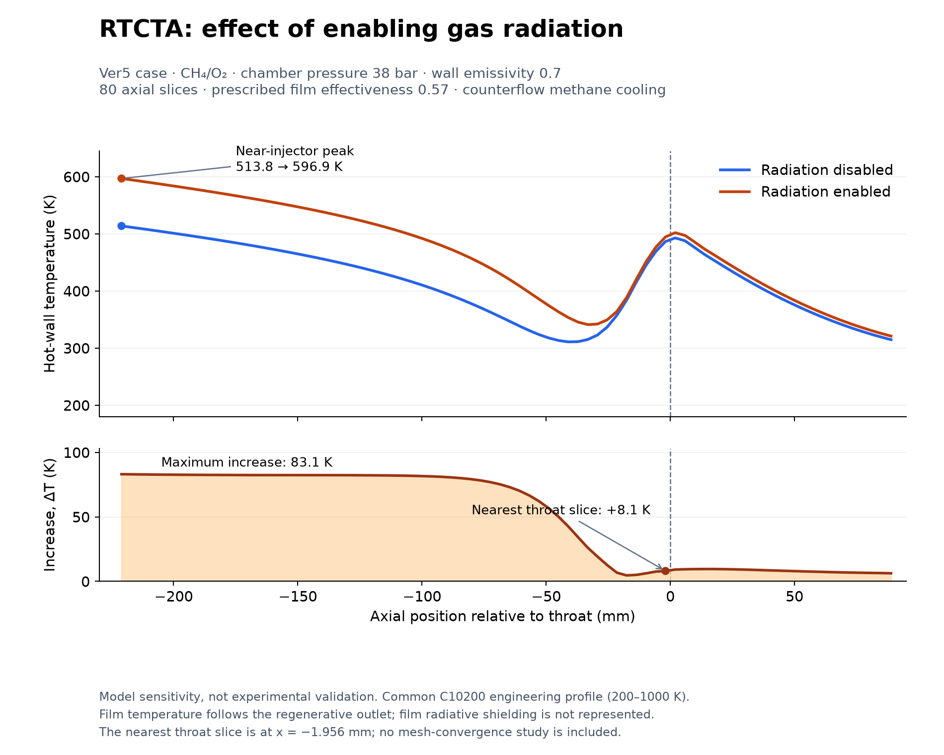
The maximum local increase is 83.1 K, at the first evaluated chamber slice. Near the throat, the increase is 8.1 K. This shows why I need the axial temperature distribution, rather than only one value at the throat.
The radiation-enabled run transfers 68.3 kW through radiation, but the total heat pickup increases by 59.0 kW. The integrated convection contribution decreases by approximately 9.3 kW as the coupled solution changes. Adding the final radiative heat load to the old convection-only result would therefore give the wrong total. These results describe this particular configuration, including its prescribed film and declared engineering material approximations. They do not mean that radiation will raise the wall temperature of every rocket engine by 83 K. Structural postprocessing was disabled for this thermal comparison, so I am not presenting a stress or life prediction from these two runs. But, I could If needed, I know that for my rocket configuration, I have to use inconel for the material and to has enough safety factor.
Comparing RTCTA with RPA
Next, I wanted to see how the gas-side calculation compared with another engineering program. I used the supplied RPA results for the SSME 40k regenerative chamber, SSME 40k calorimeter chamber, and Aestus. For this exercise, I imported the RPA contour and prescribed the local wall temperatures shown in the RPA tables. RTCTA then recalculated the heat flux using its CEA gas state, Bartz convection, and the selected radiation setting.
This is different from asking RTCTA to predict those wall temperatures. Here, the temperatures are known boundary inputs so I can examine the gas-side heat-transfer calculation.
| Case | Chamber pressure | O/F | Chamber / throat diameter | Exit area ratio | Gas radiation |
|---|---|---|---|---|---|
| SSME 40k regenerative | 20.47 MPa | 6.0 | 143.80 / 84.10 mm | 5 | Enabled |
| SSME 40k calorimeter | 10.87 MPa | 6.0 | 143.80 / 84.10 mm | 7 | Enabled |
| Aestus | 1.03 MPa | 2.05 | 210.00 / 136.00 mm | 84 | Disabled, matching the supplied table |
The SSME cases use hydrogen/oxygen. Aestus uses MMH/N2O4. Its externally radiating extension is a different mechanism from gas radiation, so a zero gas-radiation column does not mean that the extension has no outward radiative cooling.
The throat results are reasonably close:
| Case | RPA total throat flux | RTCTA total throat flux | Difference from RPA |
|---|---|---|---|
| SSME 40k regenerative | 139.83 MW/m² | 143.32 MW/m² | +2.5% |
| SSME 40k calorimeter | 91.14 MW/m² | 96.00 MW/m² | +5.3% |
| Aestus | 9.25 MW/m² | 10.24 MW/m² | +10.6% |
However, I also need to look at what happens away from the throat.
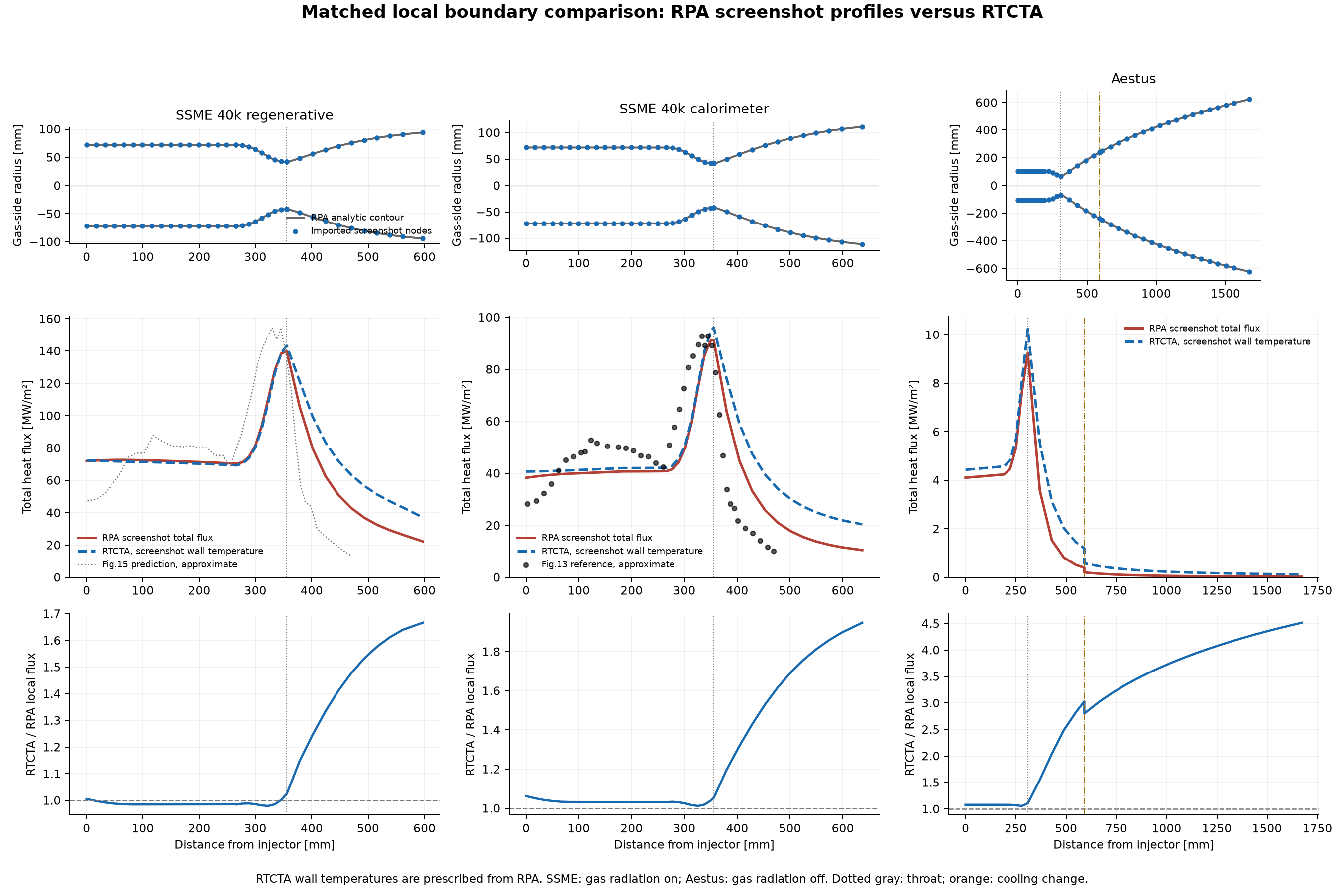
| Case | Difference in full-surface heat load | Difference over the divergent nozzle |
|---|---|---|
| SSME 40k regenerative | +11.1% | +38.2% |
| SSME 40k calorimeter | +19.4% | +51.1% |
| Aestus | +59.0% | +124.1% |
The main difference is the downstream decay: RTCTA predicts a slower decrease in heat flux. A close result at the throat does not automatically give a close total heat load over the complete nozzle.
There are several model differences to investigate. RTCTA uses Bartz, while the distributed RPA configurations select Ievlev. The screenshots do not show the selected convection relation, so the supplied tables remain the explicit reference for this comparison. Recovery-temperature and enthalpy conventions also differ. Earlier controlled calculations showed that these choices affect the results, but the screenshot comparison does not uniquely separate their contributions. Radiation itself also needs a separate check. In a matched-state comparison for the SSME 40k calorimeter geometry, RTCTA predicted approximately 47% more radiative heat than RPA. The two programs use different radiation closures and path treatments.
Comparing with the calorimeter reference
The RPA thermal-analysis document also reproduces a calorimeter reference profile in Figure 13. Figure 14 is the corresponding RPA prediction. For the regenerative case, Figure 15 is explicitly described as a predicted reference profile, followed by the RPA prediction in Figure 16. I therefore keep those two kinds of evidence separate. For the calorimeter comparison, I approximately digitized the Figure 13 curve. I also aligned its throat-based coordinate with the injector-based coordinate used by the RPA table. The SSME throat is 355.6 mm from the injector.
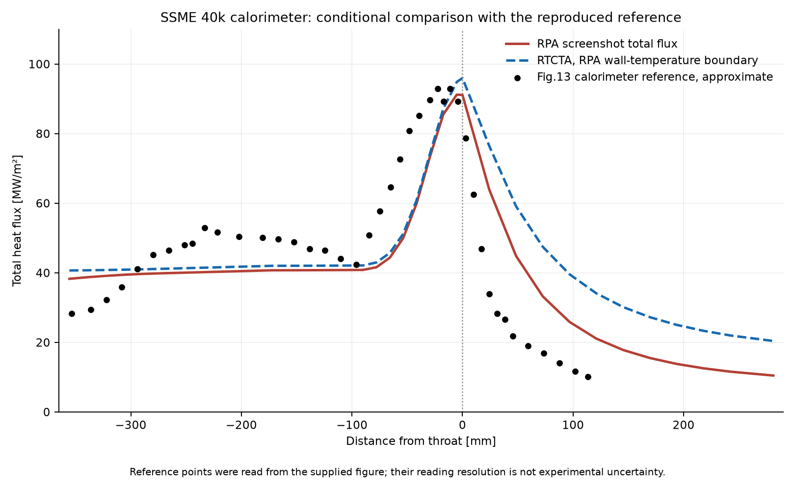
The approximate reference peak is 93 MW/m². The supplied RPA table has a maximum of 91.20 MW/m², while RTCTA gives 96.00 MW/m². The peak magnitudes are reasonably close, although the curves do not reproduce the complete chamber development, and RTCTA remains high downstream.
I consider this a useful comparison, but it is still conditional. The reference comes from a reproduced figure, not a raw digital measurement file. Its original measurement uncertainty and full test boundary conditions have not been established here. RTCTA also still uses the RPA wall temperatures as inputs. The precision with which I read the plot is not an experimental uncertainty band.
The other selected experimental target is NASA TN D-7207, run 79. That case is intended to check predicted wall temperature. Its source geometry and plotted temperature ranges have been prepared, but the tapered cooling tubes and hydrogen coolant treatment need their own supported benchmark calculation. I have not yet produced a valid RTCTA wall-temperature result for that experiment.
Conclusion
Adding radiation changed the thermal response of my saved engine case. It increased the calculated wall temperature and coolant heat pickup, and the change was not uniform along the chamber and nozzle. The RPA comparisons also helped me identify where the gas-side prediction is reasonably consistent and where more work is needed. The throat results are encouraging, while the downstream heat-flux distribution still shows substantial differences. The current base radiation model remains a homogeneous local slab approximation. It excludes soot, particles, scattering, resolved flame development, and axial radiative exchange. The wall/coolant solution does not feed heat loss back into the core gas state. The prescribed-film example does not include film radiative shielding. For me, this is part of developing the program: implement the equations, check the calculation, and compare the complete distributions. I can use the current results to investigate preliminary thermal behaviour. And TBH, this result is very promising and satsified look at how close my own program close enough to the NASA and RPA result. Even my program has one advantage compared to other, in RTCTA, I could automatically evaluate the material for my rocket. If I use this material, can it wisthstand with the operating condition? how about the structural behavior? etc.. This is a fun experiment. Ofc I also use AI (especially chatGPT) to help me such as explaining the equations, or how can I implement the equations correctly. It accelerate my learning pace and help me to connecting the dots. Because, this program combining so many concept from convection, conduction, radiation, material science, structural engineering, and ofc propulsion engineering. This is one of the most complicated program I’ve ever made.
References and implementation notes
- Marco Fabiani, Numerical Analysis of Radiative Heat Transfer in Rocket Engines, doctoral thesis, Sapienza University of Rome, defended 27 January 2026. University repository. The WSGG source data and local parallel-plate exchange basis should be distinguished from the thesis’s complete radiation modelling framework.
- RPA Thermal Analysis, July 2012 v.3, especially the convection/radiation descriptions and Figures 13–20. The distributed example configurations and supplied RPA thermal tables define the program comparisons reported here.
- NASA TN D-7207, Coolant-side heat-transfer rates for a hydrogen-oxygen rocket and a new technique for data correlation. NASA record. This is the selected wall-temperature validation target; it is not a completed RTCTA result in this article.
The main implementation files are:
| File | Role |
|---|---|
thermochemistry/cea.py | CEA gas states, transport/recovery calculation, and product composition |
resources/radiation/fabiani_wsgg.json | WSGG coefficients and their source information |
thermal/radiation.py | Input limits, table selection, weights, optical depths, exchange factor, and net radiation |
thermal/enhanced_solver.py | Slice preparation, nonlinear wall balance, coolant/wall iterations, and saved flux contributions |
thermal/resistance.py | Wall/coolant resistances and wall-temperature reconstruction |
thermal/prescribed_wall.py | Self-contained comparison-case evaluation at supplied wall temperatures |